Analysis scripts: longitudinal ESBL carriage dynamics
analysis.RmdIntroduction
This document contains reproducing analysis code which generates the tables and figures for the manuscript:
Dynamics of gut mucosal colonisation with extended spectrum beta-lactamase producing Enterobacterales in Malawi
Joseph M Lewis1,2,3,4, , Madalitso Mphasa1, Rachel Banda1, Matthew Beale4, Eva Heinz2, Jane Mallewa5, Christopher Jewell6, Nicholas R Thomson4,7, Nicholas A Feasey1,2
- Malawi Liverpool Wellcome Research Programme, Blantyre, Malawi
- Liverpool School of Tropical Medicine, Liverpool, UK
- Department of Clinical Infection, Microbiology and Immunology, University of Liverpool, Liverpool, UK
- Wellcome Sanger Institute, Hinxton, UK
- Kamuzu University of Health Sciences, Blantyre, Malawi
- University of Lancaster, Lancaster, UK
- London School of Tropical Medicine and Hygiene, London, UK
Installing and accessing data
If you just want the data, then all the data to replicate the analysis are bundled with the package. To install the package from GitHub:
The various data objects are described in the pkgdown site for
this package, and available via R in the usual way
(i.e. ?btESBL_participants brings up the definitions for
the btESBL_participants data. They are all lazy loaded so
will be available for use immediately; they all start with
btESBL_ to make it easy to choose the one you want using
autocomplete.
The analysis is available as a package vignette; this can be built when downloading the package by typing:
devtools::install_github("https://github.com/joelewis101/blantyreESBL", build_vignettes = TRUE, dependencies = TRUE )The dependencies = TRUE option will install all the
packages necessary to run the vignettes.
Alternatively the source code for the vignette is
analysis.Rmd in the vignettes/ folder of the
GitHub repo or
the pkgdown
site for this package has a rendered version.
Descriptions of participants, exposures, baseline ESBL colonisation
Setup, load packages
knitr::opts_chunk$set(
  collapse = TRUE,
  comment = "#>"
)

library(tidytree)
#> If you use the ggtree package suite in published research,
#> please cite the appropriate paper(s):
#>
#> Guangchuang Yu, Tommy Tsan-Yuk Lam, Huachen Zhu, Yi Guan. Two methods
#> for mapping and visualizing associated data on phylogeny using ggtree.
#> Molecular Biology and Evolution. 2018, 35(12):3041-3043.
#> doi:10.1093/molbev/msy194
#>
#> Guangchuang Yu. Using ggtree to visualize data on tree-like structures.
#> Current Protocols in Bioinformatics. 2020, 69:e96. doi:10.1002/cpbi.96
#>
#>
#> Attaching package: 'tidytree'
#> The following object is masked from 'package:stats':
#>
#>     filter
library(DescTools)
library(here)
#> here() starts at /Users/joelewis/R/packages/blantyreESBL
library(igraph)
#>
#> Attaching package: 'igraph'
#> The following object is masked from 'package:DescTools':
#>
#>     %c%
#> The following object is masked from 'package:tidytree':
#>
#>     parent
#> The following objects are masked from 'package:stats':
#>
#>     decompose, spectrum
#> The following object is masked from 'package:base':
#>
#>     union
library(ggraph)
#> Loading required package: ggplot2
library(dplyr)
#>
#> Attaching package: 'dplyr'
#> The following objects are masked from 'package:igraph':
#>
#>     as_data_frame, groups, union
#> The following objects are masked from 'package:stats':
#>
#>     filter, lag
#> The following objects are masked from 'package:base':
#>
#>     intersect, setdiff, setequal, union
library(tidyr)
#>
#> Attaching package: 'tidyr'
#> The following object is masked from 'package:igraph':
#>
#>     crossing
library(stringr)
library(lubridate)
#>
#> Attaching package: 'lubridate'
#> The following objects are masked from 'package:igraph':
#>
#>     %--%, union
#> The following objects are masked from 'package:base':
#>
#>     date, intersect, setdiff, union
library(purrr)
#>
#> Attaching package: 'purrr'
#> The following objects are masked from 'package:igraph':
#>
#>     compose, simplify
library(forcats)
library(glue)
library(broom)
library(ggsci)
library(bayesplot)
#> This is bayesplot version 1.10.0
#> - Online documentation and vignettes at mc-stan.org/bayesplot
#> - bayesplot theme set to bayesplot::theme_default()
#>    * Does _not_ affect other ggplot2 plots
#>    * See ?bayesplot_theme_set for details on theme setting
library(patchwork)
library(loo)
#> This is loo version 2.6.0
#> - Online documentation and vignettes at mc-stan.org/loo
#> - As of v2.0.0 loo defaults to 1 core but we recommend using as many as possible. Use the 'cores' argument or set options(mc.cores = NUM_CORES) for an entire session.
#>
#> Attaching package: 'loo'
#> The following object is masked from 'package:igraph':
#>
#>     compare
library(ggplotify)
library(pheatmap)
library(viridis)
#> Loading required package: viridisLite
library(ggtree)
#> ggtree v3.9.1 For help: https://yulab-smu.top/treedata-book/
#>
#> If you use the ggtree package suite in published research, please cite
#> the appropriate paper(s):
#>
#> Guangchuang Yu, David Smith, Huachen Zhu, Yi Guan, Tommy Tsan-Yuk Lam.
#> ggtree: an R package for visualization and annotation of phylogenetic
#> trees with their covariates and other associated data. Methods in
#> Ecology and Evolution. 2017, 8(1):28-36. doi:10.1111/2041-210X.12628
#>
#> Guangchuang Yu. Using ggtree to visualize data on tree-like structures.
#> Current Protocols in Bioinformatics. 2020, 69:e96. doi:10.1002/cpbi.96
#>
#> Guangchuang Yu.  Data Integration, Manipulation and Visualization of
#> Phylogenetic Trees (1st edition). Chapman and Hall/CRC. 2022,
#> doi:10.1201/9781003279242
#>
#> Attaching package: 'ggtree'
#> The following object is masked from 'package:tidyr':
#>
#>     expand
library(kableExtra)
#>
#> Attaching package: 'kableExtra'
#> The following object is masked from 'package:dplyr':
#>
#>     group_rows
library(blantyreESBL)

specify_decimal <- function(x, k) trimws(format(round(x, k), nsmall = k))

p.lci <- function(x,n) {
  return(binom.test(x,n)$conf.int[[1]])
}

p.uci <- function(x,n) {
  return(binom.test(x,n)$conf.int[[2]])
}

write_figs <- FALSE


if (write_figs) {
  if (!dir.exists(here("figures"))) {dir.create(here("figures"))}
  if (!dir.exists(here("tables"))) {dir.create(here("tables"))}

  if (!dir.exists(here("figures/long-modelling"))) {
    dir.create(here("figures/long-modelling"))
  }

  if (!dir.exists(here("tables/long-modelling"))) {
    dir.create(here("tables/long-modelling"))
    }
}

#render(here("vignettes/analysis.Rmd", output_dir = "~/Documents/PhD/Manuscripts/2021012_esbl_carriage/manuscript/tables_and_figs/"))
Baseline characteristics
btESBL_participants %>%
mutate(unprotected_water_source = case_when(
watersource %in% c("Unprotected well/spring",
"Surface water (including rainwater collection)") ~
"Yes",
TRUE ~ "No"),
toilet = case_when(
toilet == "Flush Toliet (any type)" ~ "Flush toilet",
TRUE ~ "Latrine or no toilet"),
watersource = case_when(
watersource %in% c("Unprotected well/spring",
"Surface water (including rainwater collection)") ~
"Unprotected",
TRUE ~ "Protected"),
keep.other = case_when(
keepanim == "No" ~ NA_character_,
keep.cattle == "Yes" ~ "Yes",
keep.mules == "Yes" ~ "Yes",
keep.sheep == "Yes" ~ "Yes",
TRUE ~ "No"),
tbongoing = if_else(is.na(tbongoing), "No", tbongoing)
) %>%
select(
c(arm,
calc_age,
ptsex,
hivstatus,
tbongoing,
hivonart,
art_time,
hivart,
hivcpt,
recieved_prehosp_ab,
pmhxrechospital,
toilet,
watersource,
watertreated,
householdchildno,
housholdadultsno,
electricityyn,
keepanim,
keep.poultry,
keep.dogs,
keep.goats,
keep.other)) -> t1.data
bind_rows(
t1.data %>%
select_if(is.character) %>%
pivot_longer(-arm) %>%
group_by(name, arm, value) %>%
tally() %>%
pivot_wider(
names_from = arm,
values_from = n,
values_fill = list(n = 0)
) %>%
filter(!is.na(value)) %>%
group_by(name) %>%
nest() %>%
mutate(p = map(
data,
~ select(.x, -value) %>%
fisher.test(simulate.p.value = TRUE) %>%
tidy() %>%
select(p.value)
)) %>%
unnest(c(data, p)) %>%
mutate(
str1 = glue('{`1`}/{sum(`1`)} ({specify_decimal(`1`*100/sum(`1`), 0)}%)'),
str2 = glue('{`2`}/{sum(`2`)} ({specify_decimal(`2`*100/sum(`2`), 0)}%)'),
str3 = glue('{`3`}/{sum(`3`)} ({specify_decimal(`3`*100/sum(`3`), 0)}%)'),
str_tot = glue(
'{`1` + `2` + `3`}/{sum(`1`) + sum(`2`) + sum(`3`)} ({specify_decimal((`1` + `2` + `3`)*100/(sum(`1`) + sum(`2`) + sum(`3`)), 0)}%)'
)
) %>%
filter(value != "No") %>%
select(name, value, str_tot, str1, str2, str3, p.value),
t1.data %>%
select(where(is.numeric) | contains("arm")) %>%
pivot_longer(-arm) %>%
group_by(name) %>% mutate(
p = kruskal.test(value ~ arm)$p.value,
median.t = median(value, na.rm = T),
lqr.t = quantile(value, 0.25, na.rm = T),
uqr.t = quantile(value, 0.75, na.rm = T),
Total = glue(
'{specify_decimal(median.t,1)} ({specify_decimal(lqr.t,1)}-{specify_decimal(uqr.t,1)})'
)
) %>%
group_by(name, arm) %>% summarise(
median = median(value, na.rm = T),
lqr = quantile(value, 0.25, na.rm = T),
uqr = quantile(value, 0.75, na.rm = T),
strz = glue(
'{specify_decimal(median,1)} ({specify_decimal(lqr,1)}-{specify_decimal(uqr,1)})'
),
p = unique(p),
Total = unique(Total)
) %>% select(name, arm, strz, p, Total) %>%
mutate(arm = paste0("str", arm)) %>%
pivot_wider(
id_cols = c(name, p, Total),
names_from = arm,
values_from = strz
) %>%
rename(p.value = p,
str_tot = Total)
) %>%
mutate(value = if_else(is.na(value), name, value)) -> t1
#> `summarise()` has grouped output by 'name'. You can override using the
#> `.groups` argument.
t1 %>%
filter(
value != "Unprotected",
value != "Latrine or no toilet",
value != "Female",
value != "ART regimen: other"
) %>%
mutate(
value = if_else(name == "hivstatus",
paste0("HIV ",str_to_title(value)), value),
value = case_when(
name == "householdchildno" ~ "Number of children",
name == "housholdadultsno" ~ "Number of adults",
name == "calc_age" ~ "Age (yr)",
name == "art_time" ~ "Months on ART",
name == "hivonart"~ "Current ART",
name == "hivcpt" ~ "Current CPT",
value == "5A" ~ "ART regimen: EFV/3TC/TDF",
# name == "tbstatus" ~ "Ever treated for TB",
name == "tbongoing" ~ "Current TB treatment",
name == "recieved_prehosp_ab" ~ "Antibiotics within 28 days<sup>†</sup>",
name == "pmhxrechospital" ~ "Hospitalised within 28 days",
name == "watertreated" ~ "Treat drinking water with chlorine",
value == "Protected" ~ "Protected water source<sup>§</sup>",
name == "keepanim" ~ "Keep animals",
name == "electricityyn" ~ "Electricty in house",
grepl("keep", name) ~ str_to_title(gsub("keep\\.","", name)),
value == "Flush toilet" ~ "Flush toilet<sup>‡</sup>",
TRUE ~ value),
# ---
name = case_when(
grepl("keep\\.", name) |
name %in% c( "householdchildno", "housholdadultsno",
"keepanim", "electricityyn") ~ "Household",
name %in% c("calc_age", "ptsex") ~ "Demographics",
name %in% c("hivstatus") ~ "HIV status",
name %in% c("tbstatus", "tbongoing") ~ "Healthcare exposure",
grepl("art", name) | grepl("cpt", name) ~ "ART status*",
name %in% c("recieved_prehosp_ab", "pmhxrechospital", "tbongoing") ~
"Healthcare exposure",
name %in% c("toilet", "watertreated", "watersource") ~ "Household",
TRUE ~ name
),
# ---
name = factor(
name,
levels = c(
"Demographics",
"HIV status",
"ART status*",
"Healthcare exposure",
"Household"
)),
value = factor(
value,
levels = c(
"Age (yr)",
"Male",
"HIV Reactive",
"Current CPT",
"Current ART",
"ART regimen: EFV/3TC/TDF",
"Months on ART",
"HIV Non Reactive",
"HIV Unknown",
"Antibiotics within 28 days<sup>†</sup>",
"Hospitalised within 28 days",
"Current TB treatment",
"Number of adults",
"Number of children",
"Keep animals",
"Poultry",
"Dogs",
"Goats",
"Other",
"Electricty in house",
"Flush toilet<sup>‡</sup>",
"Protected water source<sup>§</sup>",
"Treat drinking water with chlorine"
))) -> t1
t1 %>%
arrange(name, value) %>%
mutate(p.value = specify_decimal(p.value,3),
p.value = if_else(p.value == "0.000", "<0.001", p.value),
p.value = case_when(
value %in% c("HIV Non Reactive",
"HIV Unknown",
"Poultry",
"Dogs",
"Goats",
"Other") ~ "",
TRUE ~ p.value)) -> t1
t1 %>%
dplyr::group_by(name, .drop = TRUE) %>%
summarise(n = n()) %>%
pull(n) -> groupvar
names(groupvar) <- unique(t1$name)
indentrows <- which(t1$value %in%
c("Poultry",
"Dogs",
"Goats",
"Other"))
t1 %>%
ungroup() %>%
select(value, str1, str2, str3, p.value,str_tot) %>%
kbl(col.names =
c(
"Variable",
"Sepsis (n=225)",
"Inpatient (n=100)",
"Community (n=100)",
"p",
"Total (n = 425)"
),
escape = FALSE,
caption = "Baseline characteristics of included participants") %>%
kable_classic(full_width = F) %>%
pack_rows(index = groupvar) %>%
row_spec(indentrows, italic = TRUE ) %>%
footnote(
general = "ART = Antiretroviral therapy, CPT = Cotrimoxazole preventative therapy, EFV: Efavirenz, 3TC: Lamivudine, TDF: Tenofovir. Numeric variables are summarised as median (IQR) and categorical variables as proportions. P-values are from Fisher's exact test (categorical variables) or Kruskal-Wallace test (continuous variables) across the three groups; p-value for HIV status compares distribution of HIV reactive, non-reactive and unknown across the three groups. In smoe cases denominator may be less than the total number of participants due to missing data.",
symbol = c(
"Denominator for ART status is HIV reactive participants only",
"Excluding TB treatment and CPT",
"Flush toilet vs latrine (pit or hanging) or no toilet",
"Protected water source includes borehole, water piped into or outside dwelling or public standpipe; unprotected sources include surface water or unprotected springs."
)
)| Variable | Sepsis (n=225) | Inpatient (n=100) | Community (n=100) | p | Total (n = 425) |
|---|---|---|---|---|---|
| Demographics | |||||
| Age (yr) | 35.9 (27.8-43.5) | 40.4 (29.1-48.3) | 32.5 (24.0-38.4) | 35.6 (26.9-43.9) | |
| Male | 114/225 (51%) | 51/100 (51%) | 40/100 (40%) | 0.176 | 205/425 (48%) |
| HIV status | |||||
| HIV Reactive | 143/225 (64%) | 12/100 (12%) | 18/100 (18%) | 173/425 (41%) | |
| HIV Non Reactive | 70/225 (31%) | 77/100 (77%) | 22/100 (22%) | 169/425 (40%) | |
| HIV Unknown | 12/225 (5%) | 11/100 (11%) | 60/100 (60%) | 83/425 (20%) | |
| ART status* | |||||
| Current CPT | 98/141 (70%) | 5/12 (42%) | 7/18 (39%) | 0.008 | 110/171 (64%) |
| Current ART | 117/143 (82%) | 9/12 (75%) | 18/18 (100%) | 0.073 | 144/173 (83%) |
| ART regimen: EFV/3TC/TDF | 110/117 (94%) | 8/9 (89%) | 17/18 (94%) | 0.639 | 135/144 (94%) |
| Months on ART | 28.7 (3.7-72.6) | 35.1 (2.9-79.8) | 31.5 (13.0-79.9) | 0.698 | 29.5 (3.8-72.8) |
| Healthcare exposure | |||||
| Antibiotics within 28 days† | 60/225 (27%) | 0/100 (0%) | 0/100 (0%) | 60/425 (14%) | |
| Hospitalised within 28 days | 18/225 (8%) | 1/100 (1%) | 0/100 (0%) | 0.002 | 19/425 (4%) |
| Current TB treatment | 10/225 (4%) | 0/100 (0%) | 4/100 (4%) | 0.093 | 14/425 (3%) |
| Household | |||||
| Number of adults | 2.0 (2.0-3.0) | 3.0 (2.0-4.0) | 2.0 (2.0-4.0) | 0.907 | 3.0 (2.0-4.0) |
| Number of children | 2.0 (1.0-3.0) | 2.0 (1.0-3.0) | 2.0 (1.0-3.0) | 0.395 | 2.0 (1.0-3.0) |
| Keep animals | 71/225 (32%) | 43/100 (43%) | 15/100 (15%) | 129/425 (30%) | |
| Poultry | 46/71 (65%) | 34/43 (79%) | 10/15 (67%) | 90/129 (70%) | |
| Dogs | 18/71 (25%) | 11/43 (26%) | 9/15 (60%) | 38/129 (29%) | |
| Goats | 12/71 (17%) | 7/43 (16%) | 1/15 (7%) | 20/129 (16%) | |
| Other | 3/71 (4%) | 6/43 (14%) | 0/15 (0%) | 9/129 (7%) | |
| Electricty in house | 119/225 (53%) | 41/100 (41%) | 58/100 (58%) | 0.050 | 218/425 (51%) |
| Flush toilet‡ | 14/225 (6%) | 5/100 (5%) | 1/100 (1%) | 0.099 | 20/425 (5%) |
| Protected water source§ | 216/225 (96%) | 92/100 (92%) | 98/100 (98%) | 0.129 | 406/425 (96%) |
| Treat drinking water with chlorine | 19/225 (8%) | 5/100 (5%) | 0/100 (0%) | 0.002 | 24/425 (6%) |
| Note: | |||||
| ART = Antiretroviral therapy, CPT = Cotrimoxazole preventative therapy, EFV: Efavirenz, 3TC: Lamivudine, TDF: Tenofovir. Numeric variables are summarised as median (IQR) and categorical variables as proportions. P-values are from Fisher’s exact test (categorical variables) or Kruskal-Wallace test (continuous variables) across the three groups; p-value for HIV status compares distribution of HIV reactive, non-reactive and unknown across the three groups. In smoe cases denominator may be less than the total number of participants due to missing data. | |||||
| * Denominator for ART status is HIV reactive participants only | |||||
| † Excluding TB treatment and CPT | |||||
| ‡ Flush toilet vs latrine (pit or hanging) or no toilet | |||||
| § Protected water source includes borehole, water piped into or outside dwelling or public standpipe; unprotected sources include surface water or unprotected springs. | |||||
Exposures
 c("Amoxicillin" = "amoxy",
  "Gentamicin" = "genta",
  "Azithromycin" = "azithro",
  "TB therapy" = "tb",
  "Penicillin" = "benzy",
  "Fluconazole" = "fluco",
  "Ceftriaxone" = "cefo",
  "Amphotericin" = "ampho",
  "Quinine" = "quin",
  "Chloramphenicol" = "chlora",
  "LA" = "coart",
  "Ciprofloxacin" = "cipro",
  "Co-amoxiclav" = "coamo",
  "Artesunate" = "arte",
  "Cotrimoxazole" = "cotri",
  "Clindamycin" = "clinda",
  "Doxycycline" = "doxy",
  "Erythromycin" = "erythro",
  "Aciclovir" = "acicl",
  "Flucloxacillin" = "fluclox",
  "Metronidazole" = "metro",
  "Streptomycin" = "strepto",
  "Hospitalised" = "hosp"
  ) -> rename_lookup


btESBL_exposures %>%
  group_by(pid) %>%
  complete(assess_type = c(0:max(assess_type))) %>%
  fill(everything()) %>%
  rename(!!!rename_lookup) %>%
  ungroup() %>%
  left_join(select(btESBL_participants, pid, arm)) %>%
  mutate(arm = case_when(
    arm == 1 ~ "Sepsis",
    arm == 2 ~ "Inpatient",
    arm == 3 ~ "Community"),
    arm = factor(arm, levels = c("Sepsis", "Inpatient", "Community"))
    ) %>%
  select(-c(pid, died)) %>% #filter(arm != 3) %>%
  pivot_longer(-c(assess_type, arm)) %>%
  group_by(arm, assess_type, name) %>%
  summarise(n = n(), x = sum(value == 1), prop = x/n)  %>%
  filter(
    name %in% c(
      "Amoxicillin",
      "Ceftriaxone",
      "Ciprofloxacin",
      "Cotrimoxazole",
      "Hospitalised",
      "TB therapy",
      "Hospitalised"
    )) %>%
  ungroup() %>%
  ggplot(aes(assess_type,prop, group = name, color = name, linetype = name)) +
  geom_line(alpha = 0.8, size = 0.75) +
  facet_wrap(~ arm, ncol = 1) +
  theme_bw() +
  scale_x_continuous(breaks = c(0,5,10,15,20,25,30), limits = c(0,30))  +
  scale_linetype_manual(values = c("Amoxicillin" =  "solid",
                                   "Ceftriaxone" = "solid",
                                   "Ciprofloxacin" = "solid",
                                   "Cotrimoxazole" = "solid",
                                   "Hospitalised" = "dashed",
                                   "TB therapy" = "dotted"),
                        breaks = c("Hospitalised",
                                   "Ceftriaxone",
                                   "Cotrimoxazole",
                                   "Ciprofloxacin",
                                   "TB therapy",
                                   "Amoxicillin")) +
  scale_colour_manual(values = c("Amoxicillin" =  pal_npg()(4)[1],
                                 "Ceftriaxone" = pal_npg()(4)[2],
                                 "Ciprofloxacin" = pal_npg()(4)[3],
                                 "Cotrimoxazole" = pal_npg()(4)[4],
                                 "Hospitalised" = "black",
                                 "TB therapy" = "grey20"),
                      breaks = c("Hospitalised",
                                   "Ceftriaxone",
                                   "Cotrimoxazole",
                                   "Ciprofloxacin",
                                   "TB therapy",
                                   "Amoxicillin")) +
  theme(legend.title = element_blank()) +
  xlab("Day post enrolment") +
  ylab("Proportion") -> exp_plot
#> Joining with `by = join_by(pid)`
#> `summarise()` has grouped output by 'arm', 'assess_type'. You can override
#> using the `.groups` argument.
#> Warning: Using `size` aesthetic for lines was deprecated in ggplot2 3.4.0.
#> ℹ Please use `linewidth` instead.
#> This warning is displayed once every 8 hours.
#> Call `lifecycle::last_lifecycle_warnings()` to see where this warning was
#> generated.

if (write_figs) {
  ggsave(here("figures/long-modelling/SUP_FIG_exposures.pdf"),exp_plot,width = 8, height = 5)
  ggsave(here("figures/long-modelling/SUP_FIG_exposures.svg"),exp_plot,width = 8, height = 5)
}
exp_plot
#> Warning: Removed 3042 rows containing missing values (`geom_line()`).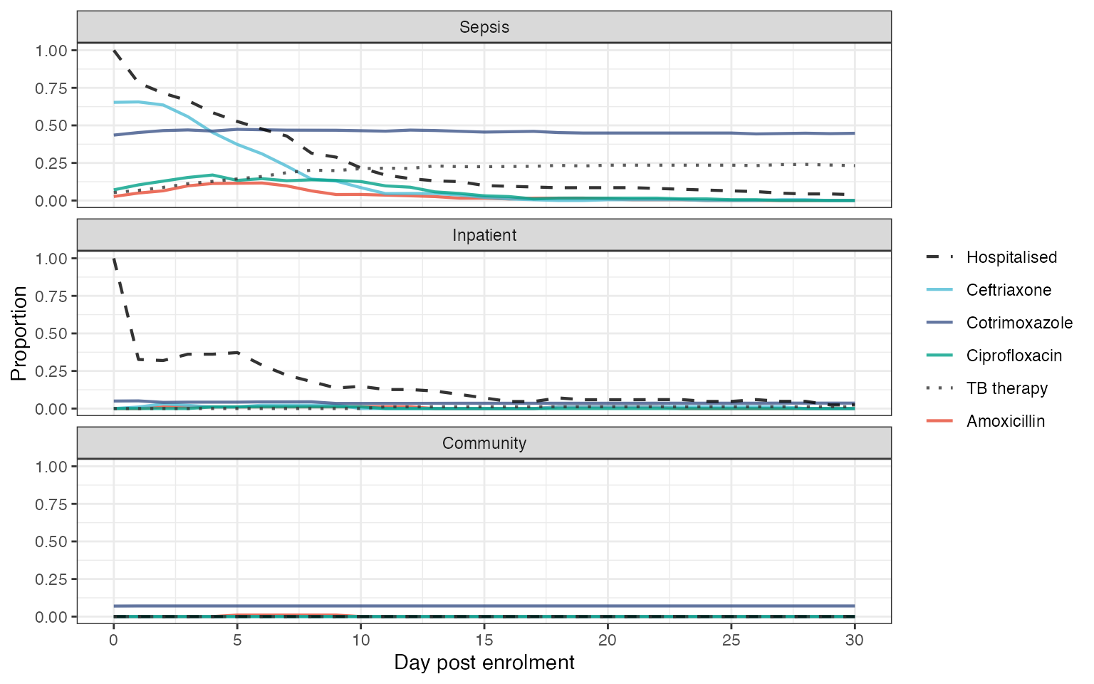
Exposures during study period. Panels show proportion of participants in each arm of the study who are hospitalised of exposed to antimicrobials on a given day
btESBL_exposures %>%
  group_by(pid) %>%
  complete(assess_type = c(0:max(assess_type))) %>%
  fill(everything()) %>%
  rename(!!!rename_lookup) %>%
  left_join(select(btESBL_participants, pid, arm)) %>%
  select(-c(assess_type, died)) %>%
  group_by(arm) %>%
  mutate('Total at risk' = 1) %>%
  pivot_longer(-c(pid, arm)) %>%
  filter(value > 0) %>%
  group_by(pid, name, arm) %>%
  summarise(pid.exp = sum(value)) %>% group_by(arm, name) %>%
  summarise(
    n.p = length(unique(pid)),
    exposure = sum(pid.exp),
    median.exp.len = median(pid.exp),
    lq.exp.len = quantile(pid.exp, 0.25),
    uq.exp.len = quantile(pid.exp, 0.75)
  )  %>%
  mutate(
    exp.len.str = paste0(
      specify_decimal(median.exp.len, 0),
      "(",
      specify_decimal(lq.exp.len, 0),
      "-",
      specify_decimal(uq.exp.len, 0),
      ")"
    ),
    exposure = as.character(exposure)
  ) %>%
  select(name, arm, n.p, exposure, exp.len.str) %>%
  mutate(
    exp.len.str =
      case_when(name == "Total" ~ "-",
                TRUE ~ exp.len.str)) %>%
  pivot_wider(
    names_from = arm,
    values_from = c(n.p, exposure, exp.len.str),
    values_fill = list(
      n.p = 0,
      exposure = "0",
      exp.len.str = "-"
    )
  ) %>%
  arrange(desc(n.p_1), desc(name)) %>%
  kable(
    col.names = c("Exposure", rep(c("Sepsis", "Inpatient", "Community"),3)),
    caption = "Antimicrobial and hospital exposure stratified by arm") %>%
  kable_classic(full_width = FALSE) %>%
  #row_spec(1, bold = TRUE) %>%
  pack_rows("Exposures", 2, 23) %>%
  add_header_above(c(" " = 1, "Number exposed" = 3, "Exposure (person-days)" = 3,
                     "Median (IQR) exposure length (days)" = 3)) %>%
  footnote(general = "TB = tuberculosis, LA =lumefantrine artemether. Median exposure length includes only those exposed. Total at risk shows the total number of participants and participant-days of follow up included in the study.")
#> Joining with `by = join_by(pid)`
#> `summarise()` has grouped output by 'pid', 'name'. You can override using the
#> `.groups` argument.
#> `summarise()` has grouped output by 'arm'. You can override using the `.groups`
#> argument.|
Number exposed
|
Exposure (person-days)
|
Median (IQR) exposure length (days)
|
|||||||
|---|---|---|---|---|---|---|---|---|---|
| Exposure | Sepsis | Inpatient | Community | Sepsis | Inpatient | Community | Sepsis | Inpatient | Community |
| Total at risk | 225 | 100 | 100 | 33797 | 14336 | 21983 | 183(63-203) | 182(97-187) | 200(185-219) |
| Exposures | |||||||||
| Hospitalised | 225 | 100 | 1 | 1727 | 500 | 1 | 5(2-10) | 2(2-7) | 1(1-1) |
| Ceftriaxone | 183 | 7 | 0 | 997 | 26 | 0 | 5(3-7) | 3(2-4) |
|
| Cotrimoxazole | 110 | 6 | 7 | 14447 | 549 | 1388 | 180(27-190) | 86(6-177) | 190(183-206) |
| Ciprofloxacin | 61 | 2 | 0 | 398 | 12 | 0 | 7(5-7) | 6(6-6) |
|
| TB therapy | 52 | 2 | 0 | 6843 | 291 | 0 | 178(58-180) | 146(133-158) |
|
| Amoxicillin | 38 | 3 | 1 | 235 | 21 | 5 | 7(5-7) | 5(5-8) | 5(5-5) |
| Fluconazole | 27 | 0 | 0 | 118 | 0 | 0 | 3(2-5) |
|
|
| Metronidazole | 24 | 2 | 0 | 148 | 10 | 0 | 6(2-7) | 5(5-5) |
|
| Artesunate | 11 | 0 | 0 | 25 | 0 | 0 | 2(2-3) |
|
|
| Co-amoxiclav | 10 | 2 | 0 | 40 | 12 | 0 | 5(2-5) | 6(6-6) |
|
| LA | 7 | 0 | 0 | 19 | 0 | 0 | 3(2-3) |
|
|
| Doxycycline | 7 | 0 | 0 | 34 | 0 | 0 | 3(2-6) |
|
|
| Erythromycin | 5 | 0 | 0 | 38 | 0 | 0 | 7(5-11) |
|
|
| Gentamicin | 4 | 0 | 0 | 15 | 0 | 0 | 4(3-5) |
|
|
| Streptomycin | 2 | 0 | 0 | 16 | 0 | 0 | 8(7-9) |
|
|
| Penicillin | 2 | 0 | 0 | 5 | 0 | 0 | 2(2-3) |
|
|
| Flucloxacillin | 2 | 0 | 0 | 5 | 0 | 0 | 2(2-3) |
|
|
| Azithromycin | 2 | 2 | 0 | 7 | 12 | 0 | 4(3-4) | 6(6-6) |
|
| Amphotericin | 2 | 0 | 0 | 8 | 0 | 0 | 4(4-4) |
|
|
| Aciclovir | 2 | 0 | 0 | 47 | 0 | 0 | 24(16-31) |
|
|
| Quinine | 1 | 0 | 0 | 1 | 0 | 0 | 1(1-1) |
|
|
| Chloramphenicol | 1 | 0 | 0 | 1 | 0 | 0 | 1(1-1) |
|
|
| Note: | |||||||||
| TB = tuberculosis, LA =lumefantrine artemether. Median exposure length includes only those exposed. Total at risk shows the total number of participants and participant-days of follow up included in the study. | |||||||||
Timing of sample collection
btESBL_stoolESBL %>%
  filter(visit != 0) %>%
  mutate(visit = paste0("Visit ", visit)) %>%
  ggplot(aes(as.numeric(t), group = as.factor(visit))) +
  geom_histogram(bins = 60) +
  facet_wrap(~ visit,
  scale = 'free_y',
  ncol = 1,
  strip.position = "right") +
  xlim(c(0, 300)) +
  theme_bw() +
  xlab("Time post enrolment (days)") +
  ylab("n") -> samp_col_dates

samp_col_dates
#> Warning: Removed 7 rows containing non-finite values (`stat_bin()`).
#> Warning: Removed 8 rows containing missing values (`geom_bar()`).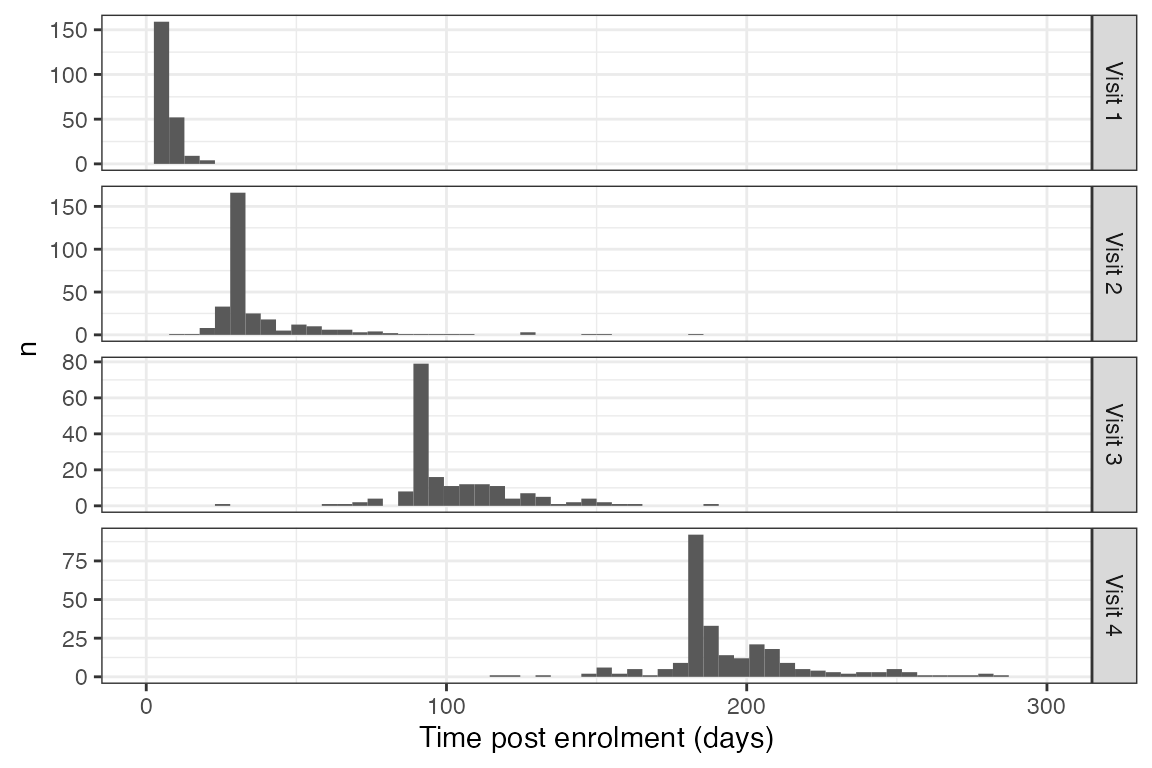
Timing of sample collection showing long tails around sample collection time.
Species of cultured bacteria from stool
btESBL_stoolorgs %>%
  mutate(
    organism =
      case_when(organism == "pantoea sp" ~ "italic('Panotea')~species",
                organism == "Gram negative bacilli" ~
                  "paste('Gram negative bacilli', '*')",
                organism == "Klebsiella pneumoniae" ~
                  "italic('Klebsiella pneumoniae')~complex",
                grepl("species", organism) ~
                  paste0(
                    "italic('",
                    gsub(" species", "", organism),
                    "')~species"
                  ),
                TRUE ~ paste0("italic('", organism, "')")),
     organism = fct_rev(fct_infreq(organism))
    ) %>%
  {ggplot(data = . , aes(organism, fill = ESBL)) +
  geom_bar() +
  coord_flip() +
  labs(y = "n",
       x = "") +
  theme_bw() +
  scale_x_discrete(labels = parse(
      text  =  unique(as.character(sort(.$organism)))
      ))
                  } -> stool_spec

stool_spec  +
  scale_fill_manual(values = viridis_pal(option = "cividis")(4)[c(3,1)]) ->
  stool_spec

stool_spec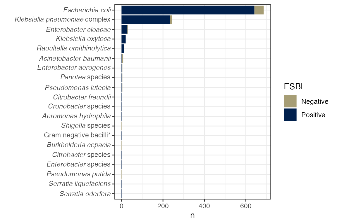
Species cultured from stool.
Antimicrobial sensitivity testins (AST) of E. coli and K. pneumoniae isolates
# sorting fn

res <- function(x) {
return(sum(x == "Resistant", na.rm = TRUE))
  }

btESBL_AST %>%
  select(-supplier_name) %>%
  pivot_longer(-organism) %>%
  mutate(value = if_else(is.na(value), "Missing", value),
         value = factor(value,
                        levels =
                          rev(c("Resistant",
                            "Intermediate",
                            "Sensitive",
                            "Missing"))),
         name = str_to_title(name)) %>%
  ggplot(aes(fct_reorder(name, value, .fun = res), fill = value)) +
  geom_bar() +
  facet_wrap(~organism, scales = "free_x") +
  coord_flip() +
  scale_fill_manual(values = viridis_pal(option = "cividis")(4),
                    breaks = c("Resistant",
                            "Intermediate",
                            "Sensitive",
                            "Missing")
                      ) +
  theme_bw() +
  labs(
    x = "Antimicrobial",
    y = "Number of isolates",
    fill = "" ) -> ast_plot

ast_plot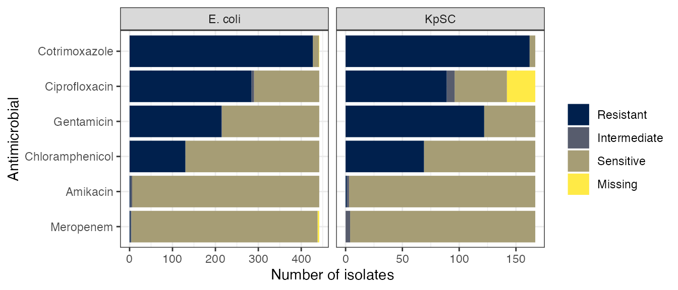
Results of antimicrobial sensitivity testing of cultured E. coli and K. pneumoniae sequence complex (KpSC) isolates using the disc diffusion method.
Plasmid replicons
btESBL_plasmidreplicons %>%
    mutate(ref_seq = gsub("_.+$","", ref_seq),
           ref_seq = gsub("\\.[0-9]","", ref_seq),
           species = if_else(
             grepl("K. pneum", species),
             "KpSC",
             species)
           # ,
           # ref_seq = case_when(
           #     grepl("Col", ref_seq) ~ "Col",
           #     grepl("rep", ref_seq) ~ "rep",
           #     grepl("^FIA", ref_seq) ~ "IncFIA",
           #     !grepl("Inc", ref_seq) ~ "Other",
           #     TRUE ~ ref_seq
           ) %>%
    filter(grepl("Inc", ref_seq)) %>%
    ggplot(aes(fct_rev(fct_infreq(ref_seq)))) +
    geom_bar() +
    coord_flip() +
    theme_bw() +
    labs(y = "Number of samples",
         x = "Plasmid replicon") +
  facet_wrap(~species, scales = "free_x") -> plasmid_replicons_plot

plasmid_replicons_plot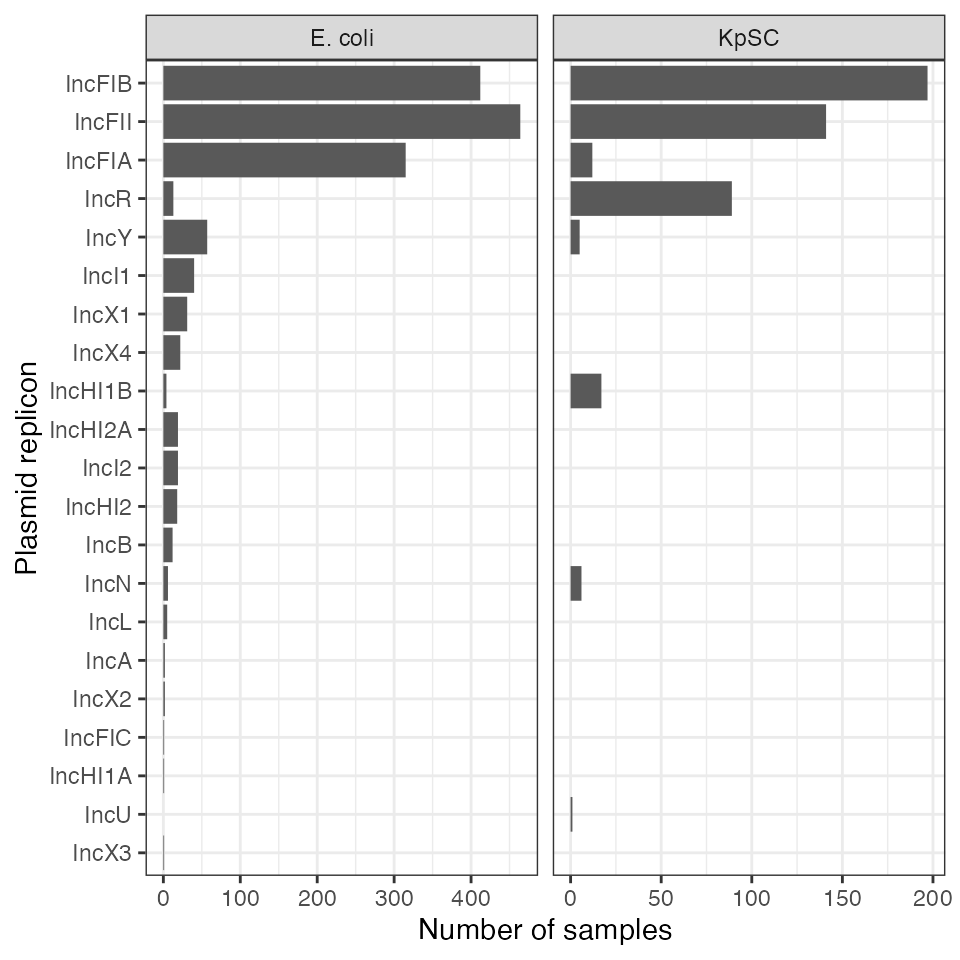
Distribution of plasmid incompatibility groups in the isolates. KpSC = Klebsiella pneumoniae sequence complex.
Baseline associations of ESBL colonisation
# helper function for univariable ods ratios

univ_or <- function(df, oc_var) {
  out <- list()
  varz <- names(df)
  varz <- varz[!grepl(oc_var, varz)]
  for (i in 1:length(varz)) {
    form <- formula(paste0(oc_var, " ~ " ,varz[i]))
    modout <- glm(formula = form, data = df, family = "binomial")
    dfout <- tidy(modout, conf.int = TRUE)
    dfout[c(2,3,6,7)] <- sapply(dfout[c(2,3,6,7)], exp)
    dfout <- dplyr::select(dfout, term, estimate, conf.low, conf.high, p.value)
    dfout <- dplyr::filter(dfout, term != "(Intercept)")
    out[[i]] <- dfout
  }
  out <- do.call(rbind, out)
  return(out)
}

# get the variables we need

btESBL_participants %>%
  select(
    pid,
    arm,
    calc_age,
    ptsex,
    hivstatus,
    hivonart,
    hivcpt,
    tbongoing,
    recieved_prehosp_ab,
    pmhxrechospital,
    watersource,
    watertreated,
    toilet,
    housholdadultsno,
    householdchildno,
    keepanim,
    enroll_date
  ) %>%
  left_join(
    btESBL_stoolESBL %>%
      filter(visit == 0) %>%
      select(pid, ESBL)
    ) %>%
  mutate(
    toilet = case_when(
      toilet == "Flush Toliet (any type)" ~ "Flush toilet",
      TRUE ~ "Latrine or no toilet"
    ),
    watersource = case_when(
      watersource %in% c(
        "Unprotected well/spring",
        "Surface water (including rainwater collection)"
      ) ~
        "Unprotected",
      TRUE ~ "Protected"
    ),
    season = case_when(
      month(enroll_date) >= 11 | month(enroll_date) <= 4 ~ "rainy",
      TRUE ~ "dry"),
    arm = case_when(
    arm == 1 ~ "Sepsis",
    arm == 2 ~ "Inpatient",
    arm == 3 ~ "Community"),
    ESBL = if_else(ESBL == "Positive", 1,0)) %>%
  mutate(across(matches("hiv|tb"), ~ if_else(is.na(.x), "No", .x))) %>%
  select(-c("pid", "enroll_date")) ->
  bl.esbl
#> Joining with `by = join_by(pid)`

# fit models

left_join(
  univ_or(bl.esbl, "ESBL") %>%
    mutate(op = paste0(specify_decimal(estimate,2), " (",
                       specify_decimal(conf.low,2), "-",
                       specify_decimal(conf.high,2), ")")
           ),
  tidy(
  glm(ESBL ~ ., data = bl.esbl, family = binomial(link = "logit")),
  conf.int = TRUE) %>%
  select( term, estimate, conf.low, conf.high, p.value) %>%
    mutate(across(!matches("term|p"), exp)) %>%
  filter(term != "(Intercept)") %>%
    mutate(op = paste0(specify_decimal(estimate,2), " (",
                       specify_decimal(conf.low,2), "-",
                       specify_decimal(conf.high,2), ")")
    ),
  by = "term",
  suffix = c("_uv", "_mv")) -> log_regESBL

# recode variables lookup vector

recode.str <- c(calc_age = "Age (per year)",
  ptsexMale = "Male sex (vs female)",
  armInpatient = "Inpatient (vs community)",
  armSepsis = "Sepsis (vs community)",

  hivstatusReactive = "HIV+ (vs HIV-)",
  hivstatusUnknown = "HIV unknown (vs HIV-)",
  hivcptYes = "CPT (vs none)",
  pmhxrechospitalYes = "Hospitalisation",
  recieved_prehosp_abYes = "Antibiotics*",
  tbongoingYes = "Current TB treatment",
  housholdadultsno = "Adults (per 1)",
  householdchildno = "Children (per 1)",
  keepanimYes = "Keep animals (vs. not)",
  `toiletLatrine or no toilet` = "Flushing toilet (vs. not)",
  watersourceUnprotected = "Unprotected water source",
  watertreatedYes = "Treat water (vs not)",
  seasonrainy = "Rainy season (vs. dry)"

  )


log_regESBL %>%
  mutate(across(matches("p\\.value"), ~ case_when(
    .x < 0.001 ~ "<0.001",
    TRUE ~ specify_decimal(.x, 3)))
  ) %>%
  select(term,op_uv, p.value_uv,
         op_mv, p.value_mv) %>%
  mutate(term = recode_factor(term, !!!recode.str, .ordered = TRUE)) %>%
   kable( col.names = c("Variable",
                        "OR (95\\% CI)",
                        "p-value",
                        "aOR (95\\% CI)",
                        "p-value"),
      caption = "Univariable and multivariable associations of ESBL colonisation at enrolment") %>%
        kable_classic(full_width = FALSE) %>%
      column_spec(2:3, bold = log_regESBL$p.value_uv < 0.05) %>%
  column_spec(4:5, bold = log_regESBL$p.value_mv < 0.05) %>%
       pack_rows("Study Arm", 1,2, bold = FALSE) %>%
       pack_rows("Demographics", 3,4, bold = FALSE) %>%
       pack_rows("HIV status", 5,8, bold = FALSE) %>%
       pack_rows("Healthcare exposure", 9,11, bold = FALSE) %>%
       pack_rows("Household", 12,17, bold = FALSE) %>%
       pack_rows("Season", 18,18, bold = FALSE) %>%
  add_header_above(c(" " = 1, "Univariable" = 2, "Multivariable" = 2)) %>%
footnote(general = "CPT = Cotrimoxazole preventative therapy, ART = antiretroviral therapy, TB = tuberculosis. Entries in bold are those for which 95% confidence intervals do not cross 1.", symbol = "Antibiotics includes TB therapy but excludes CPT.") |
Univariable
|
Multivariable
|
|||
|---|---|---|---|---|
| Variable | OR (95% CI) | p-value | aOR (95% CI) | p-value |
| Study Arm | ||||
| Inpatient (vs community) | 1.79 (1.00-3.26) | 0.054 | 1.68 (0.81-3.53) | 0.164 |
| Sepsis (vs community) | 2.45 (1.48-4.12) | <0.001 | 1.08 (0.54-2.22) | 0.822 |
| Demographics | ||||
| Age (per year) | 1.00 (0.99-1.02) | 0.709 | 1.00 (0.98-1.02) | 0.922 |
| Male sex (vs female) | 1.23 (0.84-1.82) | 0.287 | 1.44 (0.94-2.21) | 0.098 |
| HIV status | ||||
| HIV+ (vs HIV-) | 1.68 (1.09-2.59) | 0.018 | 1.21 (0.48-2.99) | 0.679 |
| HIV unknown (vs HIV-) | 0.71 (0.40-1.24) | 0.229 | 1.08 (0.54-2.16) | 0.820 |
| hivonartYes | 1.99 (1.32-3.00) | 0.001 | 1.07 (0.35-3.23) | 0.905 |
| CPT (vs none) | 2.46 (1.58-3.86) | <0.001 | 2.34 (1.00-5.66) | 0.053 |
| Healthcare exposure | ||||
| Current TB treatment | 1.02 (0.33-2.99) | 0.971 | 0.51 (0.13-1.80) | 0.300 |
| Antibiotics* | 1.81 (1.05-3.16) | 0.034 | 1.24 (0.64-2.41) | 0.528 |
| Hospitalisation | 7.87 (2.57-34.22) | 0.001 | 6.64 (1.98-30.75) | 0.005 |
| Household | ||||
| Unprotected water source | 2.43 (0.96-6.64) | 0.068 | 2.96 (1.07-8.75) | 0.040 |
| Treat water (vs not) | 1.16 (0.50-2.66) | 0.725 | 0.95 (0.37-2.37) | 0.913 |
| Flushing toilet (vs. not) | 0.72 (0.29-1.80) | 0.481 | 1.11 (0.41-3.04) | 0.842 |
| Adults (per 1) | 1.14 (0.99-1.31) | 0.064 | 1.20 (1.03-1.40) | 0.024 |
| Children (per 1) | 1.00 (0.87-1.14) | 0.979 | 0.98 (0.84-1.13) | 0.747 |
| Keep animals (vs. not) | 1.33 (0.88-2.03) | 0.176 | 1.15 (0.72-1.84) | 0.552 |
| Season | ||||
| Rainy season (vs. dry) | 2.05 (1.38-3.06) | <0.001 | 2.21 (1.40-3.50) | <0.001 |
| Note: | ||||
| CPT = Cotrimoxazole preventative therapy, ART = antiretroviral therapy, TB = tuberculosis. Entries in bold are those for which 95% confidence intervals do not cross 1. | ||||
| * Antibiotics includes TB therapy but excludes CPT. | ||||
Describing and modelling longitudinal ESBL carriage
Longitudinal carriage plot
left_join(
  btESBL_stoolESBL %>%
    group_by(arm, visit) %>%
    summarise(n = n(),
              n_esbl = sum(ESBL == "Positive")),

  btESBL_stoolESBL %>%
    left_join(btESBL_stoolorgs %>%
                filter(ESBL == "Positive") %>%
                select(lab_id,organism)) %>%
    group_by(arm, visit) %>%
    summarise(
      n_esco = sum(organism == "Escherichia coli", na.rm = TRUE),
      n_kleb = sum(organism == "Klebsiella pneumoniae", na.rm = TRUE)
    )
) %>%
  mutate(
    esbl_str = paste0(n_esbl, " (",
                      specify_decimal(n_esbl * 100 / n, 0),
                      "%)"),
    esco_str = paste0(n_esco, " (",
                      specify_decimal(n_esco * 100 / n, 0),
                      "%)"),
    kleb_str = paste0(n_kleb, " (",
                      specify_decimal(n_kleb * 100 / n, 0),
                      "%)"),
    n = as.character(n)
  ) %>%
  select(visit, arm, n, esbl_str, esco_str, kleb_str) %>%
  pivot_wider(
    id_cols = visit ,
    names_from = arm,
    values_from = c("n", "esbl_str", "esco_str", "kleb_str"),
    values_fill = "-"
  ) %>%
  select(
    visit,
    n_1,
    esbl_str_1,
    esco_str_1,
    kleb_str_1,
    n_2,
    esbl_str_2,
    esco_str_2,
    kleb_str_2,
    n_3,
    esbl_str_3,
    esco_str_3,
    kleb_str_3
  ) %>%
  mutate(
    visit = case_when(
      visit == 0 ~ "Baseline",
      visit == 1 ~ "Day 7",
      visit == 2 ~ "Day 28",
      visit == 3 ~ "Day 90",
      visit == 4 ~ "Day 180"
    )) %>%
      kable(col.names = c("Visit", rep(
        c("n", "ESBL", "E. coli", "K. pneumo"), 3
      )),
      caption = "ESBL, E. coli and K. pneumoniae prevalence in stool at study visits, stratified by study arm.") %>%
      kable_classic(full_width = FALSE) %>%
      add_header_above(c(
        " " = 1,
        "Sepsis" = 4,
        "Inpatient" = 4,
        "Community" = 4
      ))
#> `summarise()` has grouped output by 'arm'. You can override using the `.groups`
#> argument.
#> Joining with `by = join_by(lab_id)`
#> `summarise()` has grouped output by 'arm'. You can override using the `.groups`
#> argument.
#> Joining with `by = join_by(arm, visit)`|
Sepsis
|
Inpatient
|
Community
|
||||||||||
|---|---|---|---|---|---|---|---|---|---|---|---|---|
| Visit | n | ESBL | E. coli | K. pneumo | n | ESBL | E. coli | K. pneumo | n | ESBL | E. coli | K. pneumo |
| Baseline | 222 | 109 (49%) | 98 (44%) | 34 (15%) | 99 | 41 (41%) | 35 (35%) | 10 (10%) | 99 | 28 (28%) | 25 (25%) | 6 (6%) |
| Day 7 | 162 | 127 (78%) | 122 (75%) | 45 (28%) | 63 | 32 (51%) | 27 (43%) | 8 (13%) |
|
|
|
|
| Day 28 | 148 | 106 (72%) | 97 (66%) | 46 (31%) | 71 | 37 (52%) | 30 (42%) | 16 (23%) | 92 | 29 (32%) | 23 (25%) | 9 (10%) |
| Day 90 | 126 | 71 (56%) | 62 (49%) | 24 (19%) | 60 | 29 (48%) | 25 (42%) | 4 (7%) |
|
|
|
|
| Day 180 | 127 | 61 (48%) | 55 (43%) | 24 (19%) | 65 | 29 (45%) | 23 (35%) | 5 (8%) | 82 | 23 (28%) | 18 (22%) | 2 (2%) |
fills = c("#A25050","#6497b1","#7cb9b9")


cols = c("#8F2727","#03396c","#278f8f")

# get first ab exposure
btESBL_stoolESBL %>%
left_join(
    btESBL_exposures %>%
      group_by(pid) %>%
      complete(assess_type = c(0:max(assess_type))) %>%
      fill(everything()) %>% rowwise() %>%
      mutate(any_abx = any(c_across(!matches(
        "pid|assess|hosp|died"
      )) == 1)) %>%
      group_by(pid) %>%
      filter(any_abx == 1) %>%
      arrange(pid, assess_type) %>%
      slice(1) %>%
      mutate(first_ab = assess_type) %>%
      select(pid, first_ab)) %>%
  # and hospital exposure
  left_join(
    btESBL_exposures %>%
      group_by(pid) %>%
      complete(assess_type = c(0:max(assess_type))) %>%
      fill(everything()) %>%
      group_by(pid) %>%
      filter(hosp == 1) %>%
      arrange(pid, assess_type) %>%
      slice(1) %>%
      mutate(first_hosp = assess_type) %>%
      select(pid, first_hosp)) %>%
  # censor as described
  filter(
    !(arm == 2 & !is.na(first_ab) & first_ab < t),
    !(arm == 3 & !is.na(first_ab) & first_ab < t),
    !(arm == 3 & !is.na(first_hosp) & first_hosp < t)
  ) %>%
  mutate(arm = case_when(
    arm == 1 ~ "Inpatient:\nantimicrobials",
    arm == 2 ~ "Inpatient:\nno antimicrobials",
    arm == 3 ~ "Community"),
    arm = factor(arm, levels = c("Inpatient:\nantimicrobials",
                                 "Inpatient:\nno antimicrobials",
                                 "Community"))
    ) %>%
ggplot(aes(t, as.numeric(ESBL == "Positive"),
               color = as.factor(arm),
               group = as.factor(arm),
               fill = as.factor(arm))) +
  geom_smooth(size = 0.5) +
  coord_cartesian(xlim = c(0,180), ylim = c(0.1,0.9)) +
  theme_bw() +
  scale_fill_manual(values = fills) +
  scale_color_manual(values = cols) +
#  scale_color_npg() +
 #   scale_fill_npg() +
#  scale_color_manual(values = pal_lancet()(3)[c(2,1,3)]) +
 # scale_fill_manual(values = pal_lancet()(3)[c(2,1,3)]) +
  xlab("Day post enrollment") +
  ylab("ESBL-E prevalence") +
  theme(legend.title = element_blank(),
        legend.position = "top") -> ESBLprevplot
#> Joining with `by = join_by(pid)`
#> Joining with `by = join_by(pid)`
Plot number of samples collected u to D7 with estimated prevalence
btESBL_stoolESBL %>%
  mutate(arm = paste("Arm",arm)) %>%
  ggplot(aes(t)) +
  geom_bar() +
  facet_wrap(arm ~ .) +
  xlim(c(-1, 11)) +
  labs(
    x = "Day post enrollment",
    y = "Number of samples"
  ) +
  theme_bw() -> a

btESBL_stoolESBL %>%
  mutate(arm = paste("Arm",arm)) %>%
  group_by(arm, t) %>%
  summarise(
    n_tot = length(t),
    n_esbl = sum(ESBL == "Positive", na.rm = TRUE),
    prop = n_esbl / n_tot,
    lci = binom.test(n_esbl, n_tot)$conf.int[1],
    uci = binom.test(n_esbl, n_tot)$conf.int[2]
  ) %>%
  filter(t <= 10) %>%
  ggplot(aes(x = t, y = prop, ymin = lci, ymax = uci, group = arm)) +
  geom_point() +
  geom_errorbar(width = 0) +
  facet_wrap(arm ~ .) +
  labs(
    x = "Day post enrollment",
    y = "Proportion ESBL+"
  ) +
  xlim(c(-1, 11)) +
  theme_bw() -> b
#> `summarise()` has grouped output by 'arm'. You can override using the `.groups`
#> argument.

(a / b) + plot_annotation(tag_levels = "A") -> ESBLprev_uptod7_plot

ESBLprev_uptod7_plot
#> Warning: Removed 785 rows containing non-finite values (`stat_count()`).
#> Warning: Removed 2 rows containing missing values (`geom_bar()`).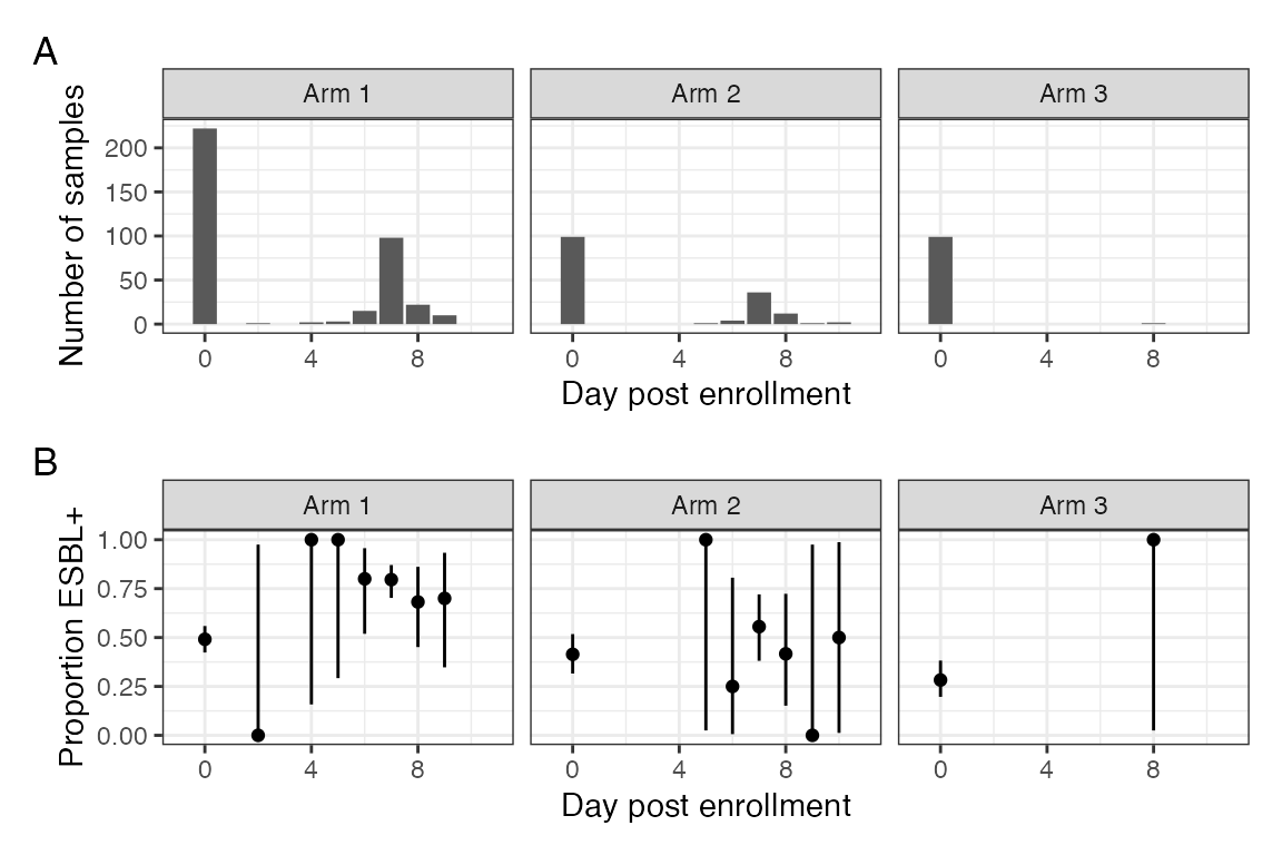
A: Number of stools samples collected per day stratified by arm. B: Proportion of samples per day in which ESBLE was identfied, stratified by arm.
if (write_figs) {
  ggsave(here("figures/long-modelling/SUP_FIG_ESBLprevD7.pdf"),
         ESBLprev_uptod7_plot,
         width = 6,
         height = 4)
  ggsave(here("figures/long-modelling/SUP_FIG_ESBLprevD7.svg"),
         ESBLprev_uptod7_plot,
         width = 6,
         height = 4)
}
Describe carriage prevalence; plot model parameters; plot predicted prevalence.
inv <- function(x) {
  return(1/x)
}

log2scale <- function(x) {
  return(log(2) * x)
}
color_scheme_set(scheme = "gray")

mcmc_areas(
  btESBL_model2posterior,
  regex_pars = "alpha|beta",
  area_method = "equal height",
  prob = 0.95,
  prob_outer = 0.99)  +
  theme_bw() +
  scale_y_discrete(
    limits = c("alphas[1]", "betas[1]", "alphas[2]", "betas[2]"),
                   labels = c("alphas[1]" = "Loss[abx]", #expression(paste(alpha,"[abx]")),
                              "alphas[2]" = "Loss[hosp]", #expression(paste(alpha,"[hosp]")),
                              "betas[1]" = "Gain[abx]", #expression(paste(beta,"[abx]")),
                              "betas[2]" = "Gain[hosp]" #expression(paste(beta,"[hosp]"))
                              ),
    expand = expansion(add = c(0.2,1))
    ) +
    labs(x = "Log HR ESBL gain/loss") -> a
#> Scale for y is already present.
#> Adding another scale for y, which will replace the existing scale.

mcmc_areas(
    btESBL_model2posterior,
    regex_pars = "alphas.2|betas.2",area_method = "equal height",
    point_est = "median", transformations = exp, prob = 0.95,
    prob_outer = 0.95) +
    theme_bw() +
  scale_y_discrete(
    limits = c( "t(betas[2])", "t(alphas[2])"),
                   labels = c(
                              "t(alphas[2])" = "Loss[hosp]",
                              "t(betas[2])" = "Gain[hosp]"
                              ),
    expand = expansion(add = c(0.2,1))
    ) -> a.1
#> Scale for y is already present.
#> Adding another scale for y, which will replace the existing scale.

mcmc_areas(
    btESBL_model2posterior,
    regex_pars = "alphas.1|betas.1",area_method = "equal height",
    point_est = "median", transformations = exp, prob = 0.95,
    prob_outer = 0.95) +
    theme_bw() +
  scale_y_discrete(
    limits = c( "t(betas[1])", "t(alphas[1])"),
                   labels = c(
                              "t(alphas[1])" = "Loss[abx]",
                              "t(betas[1])" = "Gain[abx]"
                              ),
    expand = expansion(add = c(0.2,1))
    ) +
    labs(x = "Hazard ratio  \nESBL gain/loss") -> a.2
#> Scale for y is already present.
#> Adding another scale for y, which will replace the existing scale.


mcmc_areas(
  btESBL_model2posterior,
  regex_pars = "lambda|mu",
  transformations = inv,
  area_method = "equal height",
  prob = 0.95,
  prob_outer = 0.99)  +
  theme_bw() +   #-> c #+
  scale_y_discrete(limits = c("t(lambda)", "t(mu)"),
                   labels = c("t(lambda)" = "Uncolonised", #expression(paste(lambda^'-1')),
                              "t(mu)" = "Colonised"), # expression(paste(mu^'-1'))),
  expand = expansion(add = c(0.2,1))) +
  labs(x = "Mean time in state (days)") -> b
#> Scale for y is already present.
#> Adding another scale for y, which will replace the existing scale.

mcmc_areas(
  btESBL_model2posterior,
  regex_pars = "gamma" ,
  transformations = log2scale,
  prob = 0.95,
  prob_outer = 0.99) +
  theme_bw() +   #-> c #+
  scale_y_discrete(limits = "t(gammas[1])",
                  labels = c("t(gammas[1])" = "Half life"), # expression(paste(gamma, "log(2))"))),
          #        labels = c("t(gammas[1])" = "\u03b3 log(2)"),
  expand = expansion(add = c(0.2,1))) +
  labs(x = "Antimicrobial effect  \nhalf life (days)") -> c
#> Scale for y is already present.
#> Adding another scale for y, which will replace the existing scale.

# simulated data


#cols2 = c("#ffcc80", "#a25079","#660066")

btESBL_model2simulations %>%
  mutate(abx_days = as.factor(abx_days)) %>%
    group_by(time, abx_days) %>%
    summarise(
        median = median(pr_esbl_pos),
        lq = quantile(pr_esbl_pos, 0.025)[[1]],
        uq = quantile(pr_esbl_pos, 0.975)[[1]]
    ) %>%
    mutate(abx_stop = paste0(as.character(abx_days),
                             " days \nantimicrobials")) %>%
    ggplot(aes(
        time,
        median,
        ymin = lq,
        ymax = uq,
        linetype = fct_rev(abx_stop),
        fill = fct_rev(abx_stop),
        color = fct_rev(abx_stop))
    ) +
    geom_line() + geom_ribbon(alpha = 0.4, color = NA) +
    theme_bw() +
  theme(legend.position = "top") +
  scale_color_manual(values = c(cols[1], cols[1], cols[2])) +
  scale_fill_manual(values = c(fills[1], fills[1], fills[2])) +
  scale_linetype_manual(values = c("solid", "dashed", "solid")) +
  labs(#linetype = "Antimicrobial exposure",
       #color = "Antimicrobial exposure",
       #fill = "Antimicrobial exposure",
       y = "Simulated ESBL prevalence",
       x = "Days post enrollment") +
  coord_cartesian(ylim = c(0.1,0.9)) +
  theme(legend.title = element_blank()) -> e
#> `summarise()` has grouped output by 'time'. You can override using the
#> `.groups` argument.

a <- a.1 / a.2

((ESBLprevplot + e) / (a | b | c)) +
  plot_layout(heights = c(1.5,1.5)) +
  plot_annotation(tag_levels = "A") -> markov_panel_plot

markov_panel_plot
#> `geom_smooth()` using method = 'loess' and formula = 'y ~ x'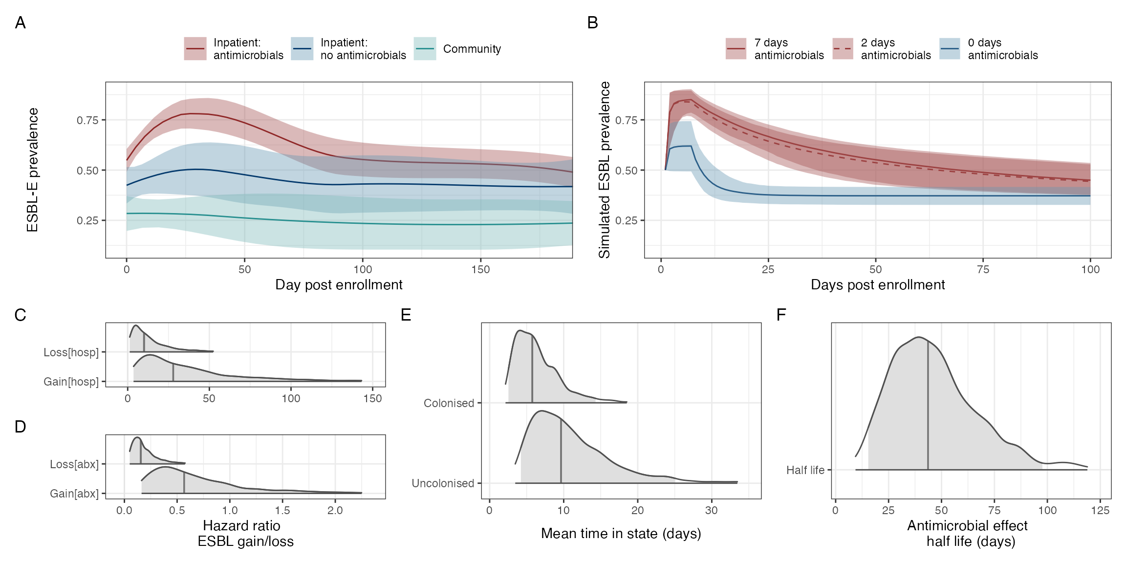
Determinants of ESBL-E carriage. A: Prevalence of ESBL-E carriage stratified by study arm. Inpatients without sepsis are censored at first antimicrobial exposure and community members censored at first antimicrobial exposure or hospital admission. Estimated prevalence and 95% confience intervals derived from a nonparametric LOESS regression with span parameter 0.8. B: Simulated probability of ESBL colonisation generated from the posterior parameter estimates of the fitted model with a starting probability of colonisation of 0.5 and seven days of hospitalisation with either seven, two, or no days antimicrobial exposure. In this model, truncated courses of antimicrobials havelittle effect on reducing ESBL-E carriage. C-E: Density plots of parameter estimates form fitted model with median (line) and 95% credible intervals (shading) shown. A: log hazard ratios of ESBL-E gain and loss for hospialisation and antimicrobial exposure: hospitalisation acts to acts to increase both acquisition and loss of ESBL-E whereas antmicrobial exposure acts to prevent loss. D: mean time in state for uncolonised and colonised states. E: Half life of decay of effecr of antimicrobials, showing that the effect of antimicrobials, in this model, acts for many days after exposure has finished.
Compare different paramaterisation of antimicrobial effect
Stepwise constant vs exponential decay.
# to

# parameter estimates from model 1 and 2

mcmc_areas(btESBL_model1posterior, regex_pars = "alpha|beta",  area_method = "equal height", prob = 0.95, prob_outer = 0.99)  +
  theme_bw() +
  scale_y_discrete(
    limits = c("ab_alpha0", "ab_beta0", "hosp_alpha1", "hosp_beta1"),
                   labels = c("ab_alpha0" = "Loss[abx]", #expression(paste(alpha,"[abx]")),
                              "hosp_alpha1" = "Loss[hosp]", #expression(paste(alpha,"[hosp]")),
                              "ab_beta0" = "Gain[abx]", #expression(paste(beta,"[abx]")),
                              "hosp_beta1" = "Gain[hosp]" #expression(paste(beta,"[hosp]"))
                              ),
    expand = expansion(add = c(0.2,1))
    ) +
    labs(x = "Log hazard ratio of ESBL gain/loss") -> a1
#> Scale for y is already present.
#> Adding another scale for y, which will replace the existing scale.

mcmc_areas(btESBL_model1posterior,
           regex_pars = "lambda|mu",
           transformations = inv,
           area_method = "equal height", prob = 0.95,
           prob_outer = 0.99)  +
  theme_bw() +   #-> c #+
  scale_y_discrete(limits = c("t(lambda)", "t(mu)"),
                   labels = c("t(lambda)" = "Uncolonised", #expression(paste(lambda^'-1')),
                              "t(mu)" = "Colonised"), # expression(paste(mu^'-1'))),
  expand = expansion(add = c(0.2,1))) +
  labs(x = "Mean time in state (days)") -> b1
#> Scale for y is already present.
#> Adding another scale for y, which will replace the existing scale.


bind_rows(
  bind_cols(as.data.frame(t(
    extract_log_lik(btESBL_model1posterior)
  )),
  select(btESBL_modeldata, pid, ESBL_stop)) %>%
    left_join(select(btESBL_participants, pid, arm), by = "pid") %>%
    pivot_longer(-c(pid, arm, ESBL_stop)) %>%
    mutate(
      pred_prob = exp(value),
      pred_state = rbinom(
        length(pred_prob),
        1,
        if_else(ESBL_stop == 1, pred_prob, 1 - pred_prob)
      )
    ) %>% group_by(arm, name) %>%
    summarise(prop = sum(pred_state == 1) / length(pred_state),
               model = "Model 1") ,

  bind_cols(as.data.frame(t(
    extract_log_lik(btESBL_model2posterior)
  )),
  select(btESBL_modeldata, pid, ESBL_stop)) %>%
    left_join(select(btESBL_participants, pid, arm), by = "pid") %>%
    pivot_longer(-c(pid, arm, ESBL_stop)) %>%
    mutate(
      pred_prob = exp(value),
      pred_state = rbinom(
        length(pred_prob),
        1,
        if_else(ESBL_stop == 1, pred_prob, 1 - pred_prob)
      )
    ) %>% group_by(arm, name) %>%
    summarise(prop = sum(pred_state == 1) / length(pred_state),
              model = "Model 2")
) %>%
  mutate(arm = case_when(
    arm == 1 ~ "Sepsis",
    arm == 2 ~ "Inpatient",
    arm == 3 ~ "Community"),
    arm = factor(arm, levels = c("Sepsis", "Inpatient", "Community"))
    )%>%
  ggplot(aes(prop, group = arm, fill = arm, color = arm)) +
  geom_density(alpha = 0.5) +
  facet_wrap( ~ model, ncol = 1) +
  geom_vline(
    data = bind_cols(as.data.frame(t(
      extract_log_lik(btESBL_model1posterior)
    )),
    select(btESBL_modeldata, pid, ESBL_stop)) %>%
      left_join(select(btESBL_participants, pid, arm), by = "pid") %>%
      pivot_longer(-c(pid, arm, ESBL_stop)) %>%
      group_by(arm) %>%
      summarise(prop = sum(ESBL_stop) / length(ESBL_stop)) %>%
      mutate(
        arm = case_when(
          arm == 1 ~ "Sepsis",
          arm == 2 ~ "Inpatient",
          arm == 3 ~ "Community"
        )
      ) ,
    aes(xintercept = prop, color = arm),
    linetype = "dashed"
  ) +
  scale_fill_manual(values = fills) +
  scale_color_manual(values = cols) +
  theme_bw() +
  labs(x = "ESBL-E prevalence") -> post_check
#> `summarise()` has grouped output by 'arm'. You can override using the `.groups`
#> argument.
#> `summarise()` has grouped output by 'arm'. You can override using the `.groups`
#> argument.

((a1 + b1 + plot_spacer() + a + b + c +  plot_layout(ncol = 3, nrow = 2))  / (post_check) ) +
  plot_annotation(tag_levels = "A") + plot_layout(heights =  c(1,1)) -> model_comp_plot

model_comp_plot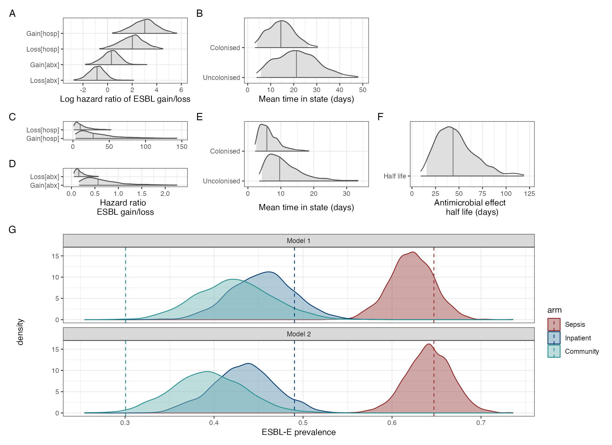
Model comparisons for models with and without an exponentially dcaying effect of antmicrobials. A-B: Parameter estimates from stepwise-constant covariate model. C-E: parameter estimates from model with exponentially-decaying effect of antinicrobial exposure. F: Posterior predictive checks of modelsm comparing model with piecewise-constant covariates (model 1) to exponentially decaying effect of antimicrobial exposure (model 2). Dashed lines show actual ESBL-E prevalence across three study arms; probability density of predicted prevalence from the two models show that model 1 tends to underestimate ESBL-E prevalence in the antimicrobial-exposed, compared to model 2.
Plot effects of antimicrobials and hospitalisation for model 2
btESBL_model2simulations_2 %>%
filter(days <= 5) %>%
  # mutate(
  #   days = if_else(
  #     days == 1, paste0(days, " day"),
  #     paste0(days, " days"))) %>%
   ggplot(aes(
     time,
     median,
     ymin = lq,
     ymax = uq,
     color = days,
     fill = days,
     group = days
   )) +
   geom_line() +
      geom_ribbon(alpha = 0.1, color = NA) +
   theme_bw() +
   facet_wrap(~ exposure) +
  scale_color_viridis(option = "magma") +
  scale_fill_viridis(option = "magma") +
  xlim(c(0,50)) +
  labs(
    x = "Time(days)",
    y = "Probability\nof ESBL colonisation",
    color = "Exposure\nduration\n(Days)",
    fill = "Exposure\nduration\n(Days)"
  )  -> a

btESBL_model2simulations_2 %>%
  group_by(days, exposure) %>%
  summarise(
    auc = AUC(time, median),
    auc.lci = AUC(time, lq),
    auc.uci = AUC(time, uq)
  ) %>%
  ggplot(aes(days, auc,
    ymin = auc.lci, ymax = auc.uci,
    linetype = exposure,
    shape = exposure
  )) +
  geom_point() +
  geom_line() +
  geom_errorbar(width = 0) +
  theme_bw() +
  labs(x = "Days of exposure",
       y = "Mean person-days\nof ESBL colonisation",
       linetype = "Exposure",
       shape = "Exposure") -> b
#> `summarise()` has grouped output by 'days'. You can override using the
#> `.groups` argument.

(a / b) + plot_annotation(tag_levels = "A") -> antimicrob_vs_hosp_plot

antimicrob_vs_hosp_plot
#> Warning: Removed 250 rows containing missing values (`geom_line()`).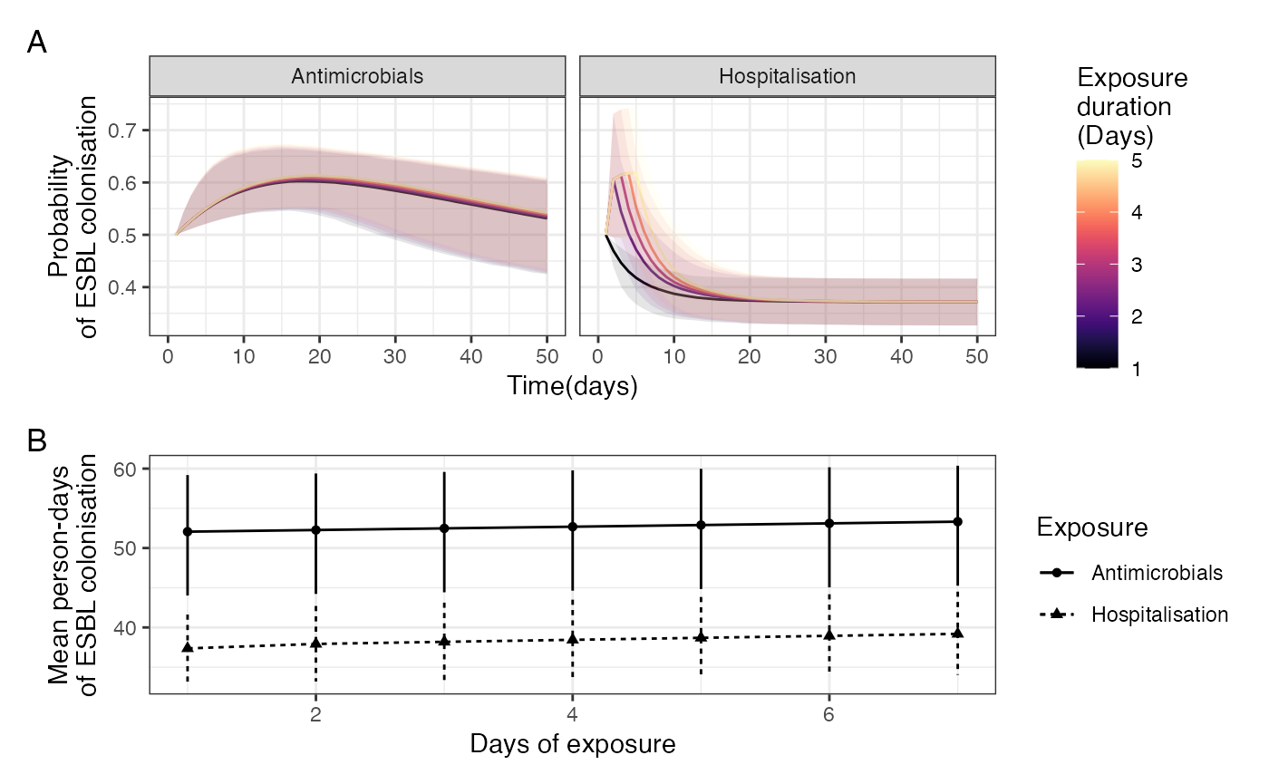
Compare model with ceftriaxone vs non-ceftraixone exposure
mcmc_intervals(btESBL_model3posterior,
               prob_outer = 0.9,
               regex_pars = "alpha|betas",
               outer_size = 1) +
  theme_bw() +
  geom_vline(xintercept = 0, linetype = "dashed") +
  scale_y_discrete(
    limits = c(
      "betas[3]", "alphas[3]",
      "betas[2]", "alphas[2]",
      "betas[1]", "alphas[1]"
    ),
    labels = c(
      "betas[3]" = expression(beta ~ "[hosp]"),
      "alphas[3]" = expression(alpha ~ "[hosp]"),
      "betas[1]" = expression(beta ~ "[CRO]"),
      "alphas[1]" = expression(alpha ~ "[CRO]"),
      "betas[2]" = expression(beta ~ "[non-CRO]"),
      "alphas[2]" = expression(alpha ~ "[non-CRO]")
    )
  ) +
  theme(axis.title.y = element_blank(), axis.text.y = element_text(size = 10)) +
  xlab("Parameter value") +
  xlim(c(-3,5)) +

mcmc_intervals(btESBL_model3posterior,
               prob_outer = 0.9,
               regex_pars = "lambda|mu",
               outer_size = 1) +
  theme_bw() +
  scale_y_discrete(limits = c("lambda", "mu"),
                   labels = c('lambda' =  expression(lambda),
                              'mu' =  expression(mu))) +
  theme(axis.title.y = element_blank(),
        axis.text.y = element_text(size = 10)) + xlab("Parameter value") +
  xlim(c(0,0.5)) +

mcmc_intervals(btESBL_model3posterior,
               prob_outer = 0.9,
               regex_pars = "gamma",
               outer_size = 1) +
  theme_bw() +
  scale_y_discrete(limits = rev(c("gammas[1]", "gammas[2]")),
                   labels = c( 'gammas[2]' =  expression(gamma~"[non-CRO]"),
                              'gammas[1]' =  expression(gamma~"[CRO]") )) +
  theme(axis.title.y = element_blank(),axis.text.y = element_text(size = 10)) +
  xlab("Parameter value") +
  xlim(c(0,200)) +
# original models

mcmc_intervals(btESBL_model2posterior,
               prob_outer = 0.9,
               regex_pars = "alpha|betas",
               outer_size = 1) +
  theme_bw() +
  geom_vline(xintercept = 0, linetype = "dashed") +
  scale_y_discrete(
    limits = c(
      "betas[2]", "alphas[2]",
      "betas[1]", "alphas[1]"
    ),
    labels = c(
      "betas[1]" = expression(beta ~ "[abx]"),
      "alphas[1]" = expression(alpha ~ "[abx]"),
      "betas[2]" = expression(beta ~ "[hosp]"),
      "alphas[2]" = expression(alpha ~ "[hosp]")
    )
  ) +
  theme(axis.title.y = element_blank(), axis.text.y = element_text(size = 10)) +
  xlab("Parameter value") +
  xlim(c(-3,5)) +

mcmc_intervals(btESBL_model2posterior,
               prob_outer = 0.9,
               regex_pars = "lambda|mu",
               outer_size = 1) +
  theme_bw() +
  scale_y_discrete(limits = c("lambda", "mu"),
                   labels = c('lambda' =  expression(lambda),
                              'mu' =  expression(mu))) +
  theme(axis.title.y = element_blank(),
        axis.text.y = element_text(size = 10)) + xlab("Parameter value") +
  xlim(c(0,0.5)) +

mcmc_intervals(btESBL_model2posterior,
               prob_outer = 0.9,
               regex_pars = "gamma",
               outer_size = 1) +
  theme_bw() +
  scale_y_discrete(limits = rev(c("gammas[1]")),
                   labels = c('gammas[1]' =  expression(gamma~"[abx]") )) +
  theme(axis.title.y = element_blank(),axis.text.y = element_text(size = 10)) +
  xlab("Parameter value") +
  xlim(c(0,200)) +
  plot_annotation(tag_levels = "A") -> cro_vs_not_model_plot
#> Scale for y is already present.
#> Adding another scale for y, which will replace the existing scale.
#> Scale for x is already present.
#> Adding another scale for x, which will replace the existing scale.
#> Scale for y is already present.
#> Adding another scale for y, which will replace the existing scale.
#> Scale for x is already present.
#> Adding another scale for x, which will replace the existing scale.
#> Scale for y is already present.
#> Adding another scale for y, which will replace the existing scale.
#> Scale for x is already present.
#> Adding another scale for x, which will replace the existing scale.
#> Scale for y is already present.
#> Adding another scale for y, which will replace the existing scale.
#> Scale for x is already present.
#> Adding another scale for x, which will replace the existing scale.
#> Scale for y is already present.
#> Adding another scale for y, which will replace the existing scale.
#> Scale for x is already present.
#> Adding another scale for x, which will replace the existing scale.
#> Scale for y is already present.
#> Adding another scale for y, which will replace the existing scale.
#> Scale for x is already present.
#> Adding another scale for x, which will replace the existing scale.

cro_vs_not_model_plot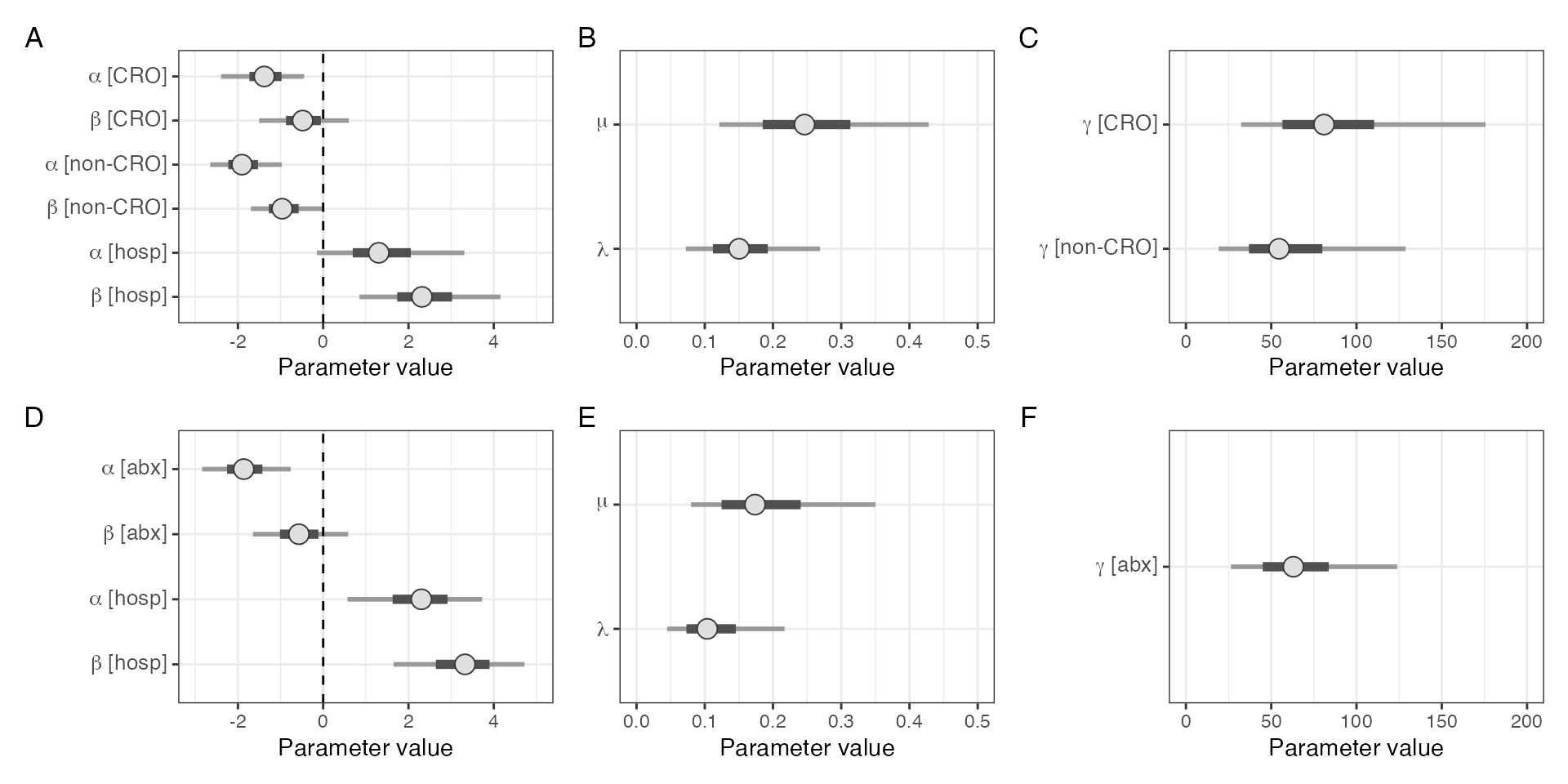
Parameter estimates from model considering ceftriaxone (CRO) exposure seperately to all other antimicrobials (A-C) versus all antimicrobials together (D-F).
Table of model parameter values
mcmc_intervals_data(
  btESBL_model2posterior,
  pars = c(
    "alphas[1]",
    "betas[1]",
    "alphas[2]",
    "betas[2]",
    "gammas[1]",
    "lambda",
    "mu"
  ),
  transformations = list(
    "alphas[1]" = exp,
    "betas[1]" = exp,
    "alphas[2]" = exp,
    "betas[2]" = exp,
    "gammas[1]" = log2scale,
    "lambda" = inv,
    "mu" = inv
  ),
  prob_outer = 0.95
) %>%
  select(parameter, ll,m,hh) %>%
  mutate(stri = glue('{specify_decimal(m,2)} ({specify_decimal(ll,2)}-{specify_decimal(hh,2)})'),
         parameter2 = case_when(
           grepl("alpha", parameter)  ~"Hazard ratio ESBL-E Loss",
           grepl("beta", parameter)  ~"Hazard ratio ESBL-E Gain",
           grepl("gamma", parameter)  ~"Half life of effect (days)",
           grepl("lambda", parameter)  ~"Colonised (days)",
           grepl("mu", parameter)  ~"Uncolonised (days)",
  ),
  parameter = factor(parameter, levels = c("t(alphas[1])",
                                           "t(betas[1])",
                                           "t(gammas[1])",
                                           "t(alphas[2])",
                                           "t(betas[2])",
                                           "t(lambda)",
                                           "t(mu)"))) %>%
  arrange(parameter) %>%
  select(parameter2, stri) %>%


kable(
  col.names = c("Variable", "Value"),
  caption = "Parameter estimates (and 95% confidence intervals) from model 2") %>%
  kable_classic(full_width = FALSE) %>%
  pack_rows("Effect of Antibacterials", 1,3) %>%
  pack_rows("Effect of Hospitalisation", 4,5) %>%
  pack_rows("Mean time in state", 6,7) %>%
footnote(general = "Hazard ratios are the exponential of the parameters alpha and beta in the model; half life is equal to log(2) multiplied by gamma; mean time in state assumes all other covariates are equal to zero and is then the reciprocal of lambda or mu.")| Variable | Value |
|---|---|
| Effect of Antibacterials | |
| Hazard ratio ESBL-E Loss | 0.16 (0.05-0.58) |
| Hazard ratio ESBL-E Gain | 0.57 (0.16-2.25) |
| Half life of effect (days) | 43.67 (15.42-97.66) |
| Effect of Hospitalisation | |
| Hazard ratio ESBL-E Loss | 10.01 (1.24-52.34) |
| Hazard ratio ESBL-E Gain | 27.82 (3.60-143.18) |
| Mean time in state | |
| Colonised (days) | 9.65 (4.22-25.07) |
| Uncolonised (days) | 5.76 (2.54-14.30) |
| Note: | |
| Hazard ratios are the exponential of the parameters alpha and beta in the model; half life is equal to log(2) multiplied by gamma; mean time in state assumes all other covariates are equal to zero and is then the reciprocal of lambda or mu. | |
Compare out-of-sample prediction with loo
# compare model 1 and model 2 with loo

ll_m1 <- extract_log_lik(btESBL_model1posterior, merge_chains = FALSE)
r_eff_m1 <- relative_eff(exp(ll_m1))

ll_m2 <- extract_log_lik(btESBL_model2posterior, merge_chains = FALSE)
r_eff_m2 <- relative_eff(exp(ll_m2))
loo_mod1 <- loo(ll_m1, r_eff = r_eff_m1)
loo_mod2 <- loo(ll_m2, r_eff = r_eff_m2)
loo_compare(loo_mod1, loo_mod2)
#>        elpd_diff se_diff
#> model2   0.0       0.0
#> model1 -10.5       4.2
Contig cluster analysis
Contig cluster associations with lineage and genus
# contig clusters: species distn -------------------------------------

btESBL_contigclusters %>% filter(clstr_size > 1) %>%
  mutate(clstr_name = fct_rev(fct_infreq(clstr_name)),
         species = if_else(species == "K. pneumoniae",
                           "K. pneumoniae\ncomplex", species),
         species = fct_rev(as.factor(species))) %>%
  group_by(species, clstr_name) %>%
  tally() %>%
  mutate(n = if_else(species == "E. coli", n,-n)) %>%
  ggplot(aes(x = clstr_name, y = n, fill = species)) +
  geom_bar(stat = "identity") +
  coord_flip() +
  theme_bw() +
  scale_y_continuous(breaks = c(-20, 0, 20, 40),
                     labels = as.character(c(20, 0, 20, 40))) +
  theme(
    legend.position = "bottom",
    legend.title = element_blank(),
    axis.text = element_text(size = 6)) +
      scale_fill_manual(values = viridis_pal()(4)[c(3,2)]) +
  labs(x = "") ->
  contigs_species_distnplot

# # map to tree

btESBL_contigclusters %>% arrange(desc(clstr_size)) %>%
  filter(clstr_size > 4) %>%
  select(lane, clstr_name) %>%
  bind_rows(
  btESBL_contigclusters %>%
  filter(clstr_size <= 4) %>%
  mutate(clstr_name = "Other") %>%
  select(lane, clstr_name)) %>%
  pivot_wider(
    id_cols = lane,
    names_from = clstr_name,
    values_from = clstr_name,
    values_fn = length,
    values_fill = 0
  ) %>%
  mutate(across(where(is.numeric), ~ as.character(if_else(.x > 0, 1, 0)))) %>%
  as.data.frame() -> clst.onehot

rownames(clst.onehot) <- clst.onehot$lane


ggtree(btESBL_coregene_tree_esco) %>%
  gheatmap((clst.onehot[-c(1, ncol(clst.onehot))]),
           font.size = 2.5,
           color = NA,
           width = 3,
           colnames = TRUE,
           colnames_angle = 90,
           colnames_offset_y = 10,
           colnames_position = "top",
           hjust = 0
  ) +
  ylim(c(0, 570)) +
  theme(legend.position = "none") +
 scale_fill_manual(values = c( "lightgrey", viridis_pal()(4)[1]) ) +
  theme(plot.margin = unit(c(0.5,0.5,0,0.5), units = "cm")) ->
  contigclusters_map_to_tree_esco
#> Scale for y is already present.
#> Adding another scale for y, which will replace the existing scale.
#> Scale for fill is already present.
#> Adding another scale for fill, which will replace the existing scale.

ggtree(tree_subset(btESBL_coregene_tree_kleb, 210,
                           levels_back = 0)) %>%
  gheatmap((clst.onehot[-c(1,ncol(clst.onehot))]),
           font.size = 2.5,
           colnames = FALSE,
           color = NA,
           width = 3,
  ) +
  scale_fill_manual(values = c( "lightgrey", viridis_pal()(4)[1]))  +
  theme(legend.position = "none") +
  theme(plot.margin = unit(c(0,0.5,0.5,0.5), units = "cm")) ->
  contigclusters_map_to_tree_kleb
#> Scale for y is already present.
#> Adding another scale for y, which will replace the existing scale.
#> Scale for fill is already present.
#> Adding another scale for fill, which will replace the existing scale.

(
    (
      (contigs_species_distnplot |
         (contigclusters_map_to_tree_esco / contigclusters_map_to_tree_kleb +
            plot_layout(heights = c(2.8,1)))) +
        plot_layout(widths = c(1,3))
     )
)  + plot_annotation(tag_levels = "A") ->
  species_lineage_mge_association

species_lineage_mge_association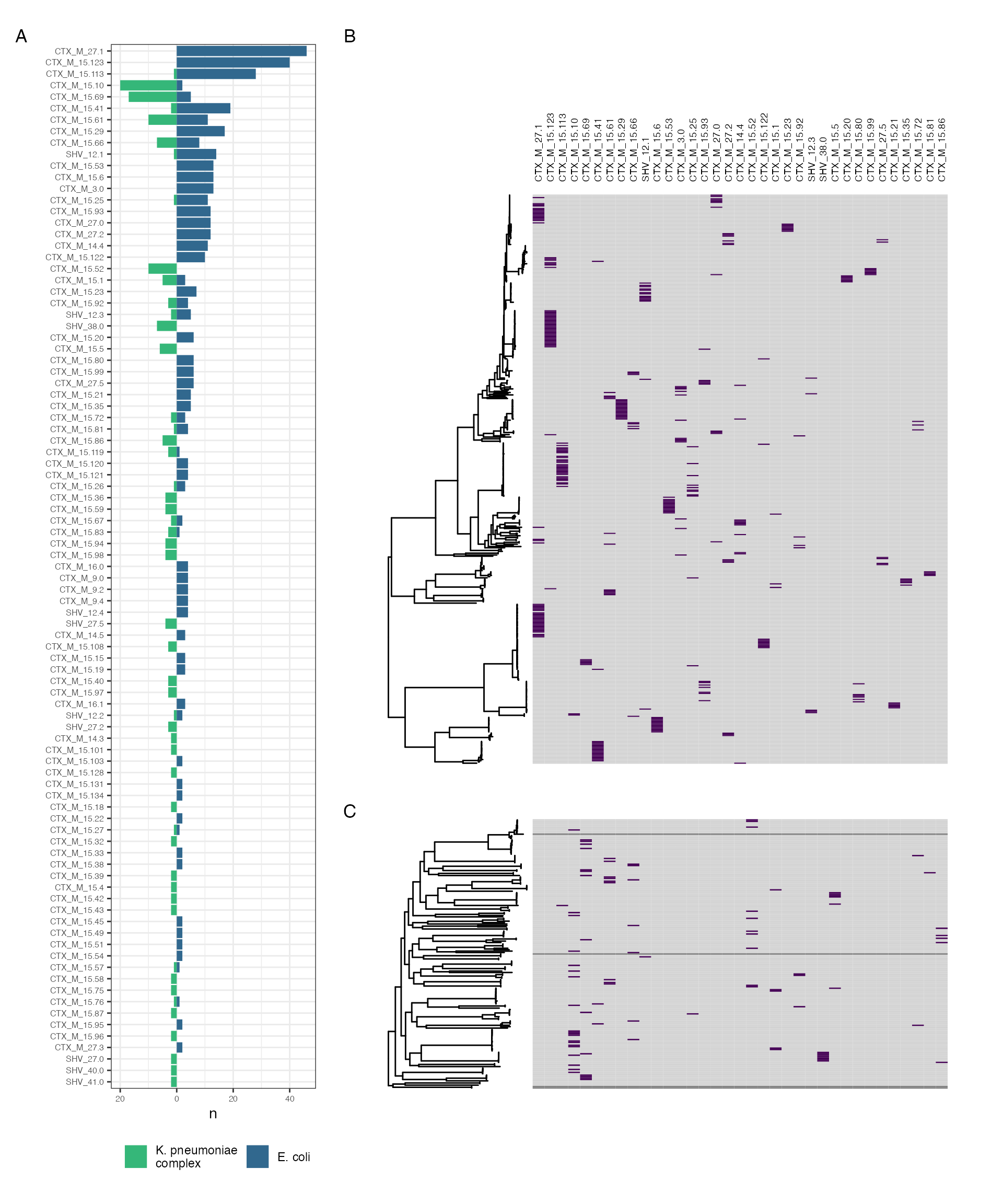
Distribution of contig-clusters between and within genera. (A) shows distribution of contig clusters by genus. (B-C) show contig-cluster presence (purple)-absence (grey) mapped back to core gene maximum likelihood phylogeny for E. coli (B) and K. pneumoniae subsp. pneumoniae (C)
Contig cluster basic statistics
btESBL_contigclusters %>%
    group_by(clstr_name) %>%
     filter(clstr_size > 1) %>%
    arrange(clstr_name, clstr_rep) %>%
    mutate(clstr_iden = clstr_iden / 100,
           clstr_cov = clstr_cov/100, clstr_size2 = clstr_size,
           clstr_rep_size = log10(last(length)/1000),
           length = log10(length/1000)) %>%
               ungroup() %>%
               # select(-length) %>%
               pivot_longer(-c(id,
                               lane,
                               clstr_rep,
                               clstr_name,
                               species,
                               gene,
                               clstr_size)) %>%
  mutate(name  = recode_factor(name,
    "clstr_size2" = "Number of samples in cluster",
    "clstr_rep_size" = "Log (base 10) length (kBases) of cluster representative sequence",
      "clstr_iden" = "Distribution of sample sequence identity to cluster representative sequence",
      "clstr_cov" = "Distribution of sample sequence coverage of cluster representative sequence",
      "length" = "Distributrion of log (base 10) sample sequence length (kBases)"),
    .ordered = TRUE) %>%
  ggplot(aes(fct_reorder(clstr_name, desc(clstr_size)), value)) +
  geom_boxplot(outlier.shape = NA) +
  facet_wrap( ~ name, ncol = 1, scales = "free_y") + theme_bw() + theme(axis.text.x = element_text(
    angle = 90,
    hjust = 1,
    size = 6
  )) +
  labs(x = "Cluster identifier", y = "") -> esbl_contig_stats

esbl_contig_stats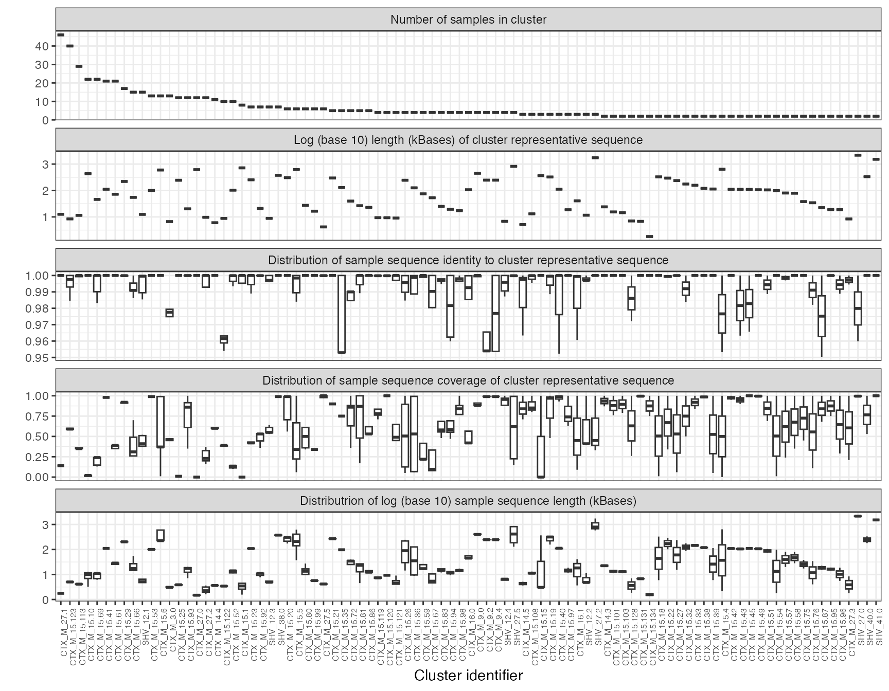
Size, representative cluster length, distribution of coverage and sequence identity of ESBL-contig clusters
popPUNK cluster analysis
popPUNK clusters mapped to phylogeny
btESBL_sequence_sample_metadata %>%
  select(lane, Cluster) %>%
  rename(Taxon = lane) %>%
  filter(grepl("K", Cluster)) %>%
  group_by(Cluster) %>%
  mutate(clst_size = n(),
         Cluster = fct_rev(fct_reorder(Cluster, clst_size))) %>%
#  select(Taxon, Cluster) %>%
  arrange(desc(clst_size)) %>%
  ungroup() %>%
  select(-clst_size) %>%
  pivot_wider(id_cols = Taxon,
              names_from = Cluster,
              values_from = Cluster,
              values_fn = length,
              values_fill = 0) %>%
  mutate(across(everything(), as.character)) %>%
  as.data.frame() -> pp.onehot.k

btESBL_sequence_sample_metadata %>%
  select(lane, Cluster) %>%
  rename(Taxon = lane) %>%
  filter(grepl("E", Cluster)) %>%
  group_by(Cluster) %>%
  mutate(clst_size = n(),
         Cluster = fct_rev(fct_reorder(Cluster, clst_size))) %>%
#  select(Taxon, Cluster) %>%
  arrange(desc(clst_size)) %>%
  ungroup() %>%
  select(-clst_size) %>%
  pivot_wider(id_cols = Taxon,
              names_from = Cluster,
              values_from = Cluster,
              values_fn = length ,
              values_fill = 0) %>%
  mutate(across(everything(), as.character)) %>%
  as.data.frame() -> pp.onehot.e

rownames(pp.onehot.e) <- pp.onehot.e$Taxon
rownames(pp.onehot.k) <- pp.onehot.k$Taxon

ggtree(btESBL_coregene_tree_esco) %>%
  gheatmap((pp.onehot.e[-1]),
           font.size = 2,
           color = NA,
           width = 3,
           colnames = TRUE,
           colnames_angle = 90,
           colnames_offset_y = 10,
           colnames_position = "top",
           hjust = 0
  ) +
  ylim(c(0, 500)) +
  theme(legend.position = "none") +
 scale_fill_manual(values = c( "lightgrey", viridis_pal()(4)[1]) )  ->
  pp.maptotree.e
#> Scale for y is already present.
#> Adding another scale for y, which will replace the existing scale.
#> Scale for fill is already present.
#> Adding another scale for fill, which will replace the existing scale.

ggtree(tree_subset(btESBL_coregene_tree_kleb, 210,
                           levels_back = 0)) %>%
  gheatmap((pp.onehot.k[-1]),
           font.size = 2,
           color = NA,
           width = 3,
           colnames = TRUE,
           colnames_angle = 90,
           colnames_offset_y = 10,
           colnames_position = "top",
           hjust = 0
  ) +
  ylim(c(0, 200)) +
  theme(legend.position = "none") +
 scale_fill_manual(values = c( "lightgrey", viridis_pal()(4)[1]) )  ->
  pp.maptotree.k
#> Scale for y is already present.
#> Adding another scale for y, which will replace the existing scale.
#> Scale for fill is already present.
#> Adding another scale for fill, which will replace the existing scale.

(pp.maptotree.e / pp.maptotree.k) +
  plot_annotation(tag_levels = "A") ->
  pp.maptotree


if (write_figs) {
  ggsave(here("figures/long-modelling/SUPP_FIG_popunk_maptotree.pdf"),
         pp.maptotree,
         width = 12,
         height = 10)
  ggsave(here("figures/long-modelling/SUPP_FIG_popunk_maptotree.svg"),
         pp.maptotree,
         width = 12,
         height = 10)
}

pp.maptotree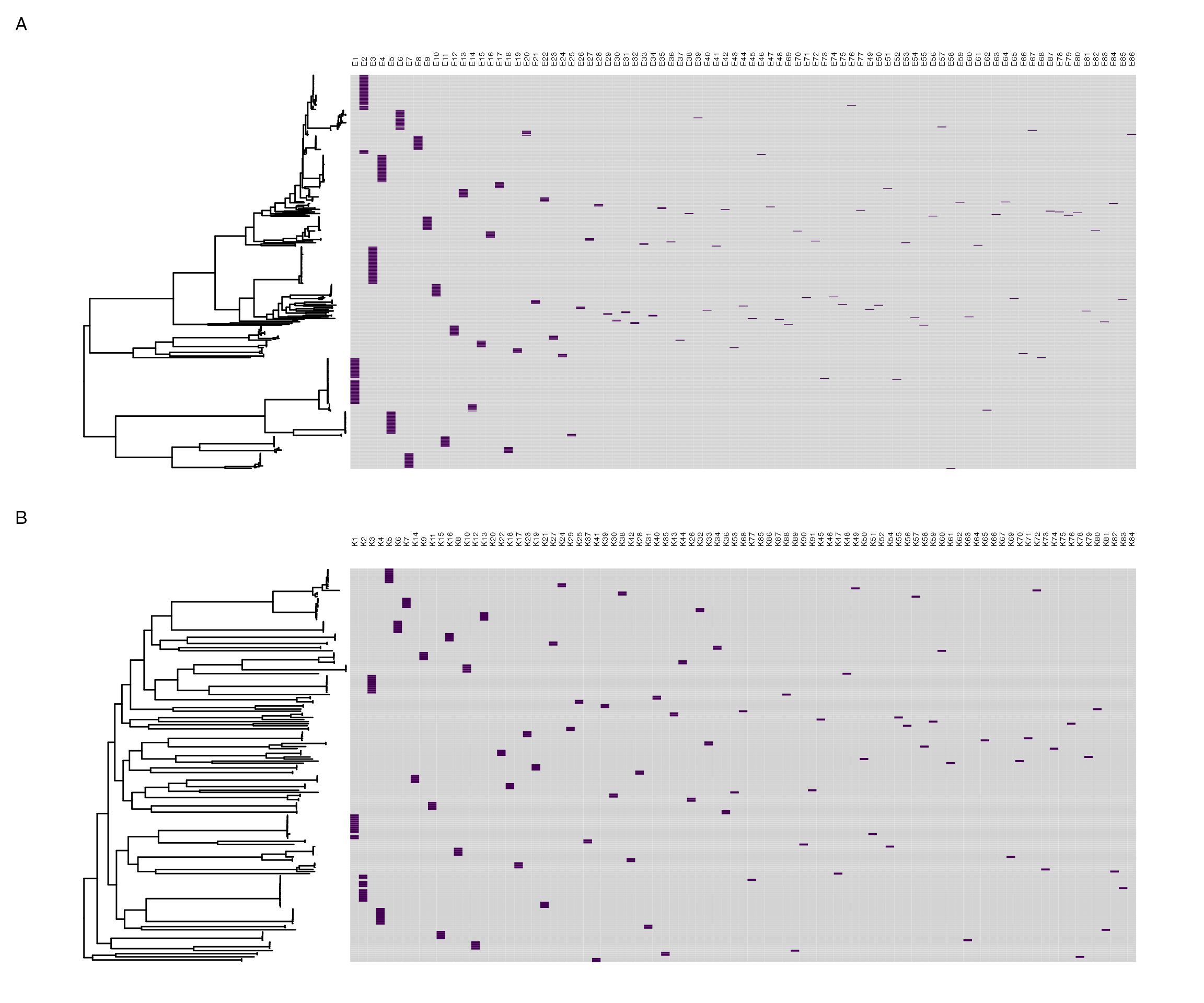
PopPUNK clusters mapped to core gene maximum-likelihood phylogeny
Within-participant temporal correlation of SNP cluster, contig and popPUNK clusters
# prepare list column tibble

btESBL_snpdists_esco %>%
  pivot_longer(-sample) %>%
  rename("sample.x" = "sample",
         "sample.y" = "name",
         "snpdist_esco" = "value") %>%
  left_join(
    select(btESBL_sequence_sample_metadata, lane, supplier_name) %>%
      rename("lab_id.x" = "supplier_name"),
    by = c("sample.x" = "lane")) %>%
  left_join(
    select(btESBL_sequence_sample_metadata, lane, supplier_name) %>%
      rename("lab_id.y" = "supplier_name"),
    by = c("sample.y" = "lane")) %>%
  group_by(lab_id.x, lab_id.y) %>%
  slice(1) %>%
  mutate(same_snpclust_esco = snpdist_esco <= 5) -> snpdist.e.long

btESBL_snpdists_kleb  %>%
  pivot_longer(-sample) %>%
  rename("sample.x" = "sample",
         "sample.y" = "name",
         "snpdist_kleb" = "value") %>%
  left_join(
    select(btESBL_sequence_sample_metadata, lane, supplier_name) %>%
      rename("lab_id.x" = "supplier_name"),
    by = c("sample.x" = "lane")) %>%
  left_join(
    select(btESBL_sequence_sample_metadata, lane, supplier_name) %>%
      rename("lab_id.y" = "supplier_name"),
    by = c("sample.y" = "lane")) %>%
  group_by(lab_id.x, lab_id.y) %>%
  slice(1) %>%
  mutate(same_snpclust_kleb = snpdist_kleb <= 5) -> snpdist.k.long

# make list-column df -----------------------------------------------------


btESBL_stoolESBL %>%
  left_join(
    btESBL_stoolorgs %>%
      filter(ESBL == "Positive") %>%
      select(lab_id, organism),
            by = "lab_id") %>%
  nest(orgs = organism) %>%
  left_join(
    select(btESBL_sequence_sample_metadata, supplier_name, Cluster),
    by = c("lab_id" = "supplier_name")
  ) %>%
  nest(pp_clust = Cluster) %>%
  left_join(
    btESBL_contigclusters %>%
      left_join(
        select(btESBL_sequence_sample_metadata , lane, supplier_name)
      ) %>%
      select(supplier_name, clstr_name),
    by = c("lab_id" = "supplier_name")
  ) %>%
  nest(contig_clust = clstr_name) %>%
  left_join(
    select(btESBL_sequence_sample_metadata, lane, supplier_name),
    by = c("lab_id" = "supplier_name")
  ) %>%
  nest(lanes = lane) -> samples
#> Joining with `by = join_by(lane)`

samples %>%
  full_join(samples, by = character())  %>%
  filter(lab_id.x != lab_id.y) %>%
  mutate(delta_t =
           interval(data_date.x, data_date.y) / days(1)) %>%
  filter(delta_t >= 0) -> samples
#> Warning: Using `by = character()` to perform a cross join was deprecated in dplyr 1.1.0.
#> ℹ Please use `cross_join()` instead.
#> This warning is displayed once every 8 hours.
#> Call `lifecycle::last_lifecycle_warnings()` to see where this warning was
#> generated.
# compare presence absence of clusters

samples %>%
  mutate(esbl.x.and.y = ESBL.x == "Positive" &
           ESBL.y == "Positive") %>%
  #compare ESCO poppunk clusters between x and y
  # and add variables for e coli cluster and presence/absence
  # e coli to later remove isolates that weren't sequenced
  mutate(
    same.esco.poppunk.xandy =
      map2(pp_clust.x,
           pp_clust.y,
           ~ .x$Cluster[grepl("E", .x$Cluster)] %in%
             .y$Cluster[grepl("E", .y$Cluster)]) %>%
      map_lgl(any),
    # flags for existence of poppunk clusters
    esco.poppunk.cluster.exists.x =
      map(pp_clust.x, ~ grepl("E", .x$Cluster)) %>%
      map_lgl(any),
    esco.poppunk.cluster.exists.y =
      map(pp_clust.y, ~ grepl("E", .x$Cluster)) %>%
      map_lgl(any),
    # flag for existence of esco
    esco.exists.x =
      map_lgl(orgs.x, ~ any(grepl("coli", .x$organism))),
    esco.exists.y =
      map_lgl(orgs.y,  ~ any(grepl("coli", .x$organism))),
    same.esco.xandy = esco.exists.x & esco.exists.y,
    # contig clusters
    same.contig.cluster =
      map2(contig_clust.x,
           contig_clust.y,
           ~ .x$clstr_name %in%
             .y$clstr_name) %>%
      map_lgl(any)
  ) %>%
  # same but for klebs
  mutate(
    same.kleb.poppunk.xandy =
      map2(pp_clust.x,
           pp_clust.y,
           ~ .x$Cluster[grepl("K", .x$Cluster)] %in%
             .y$Cluster[grepl("K", .y$Cluster)]) %>%
      map_lgl(any),
    # flags for existence of poppunk clusters
    kleb.poppunk.cluster.exists.x =
      map(pp_clust.x, ~ grepl("K", .x$Cluster)) %>%
      map_lgl(any),
    kleb.poppunk.cluster.exists.y =
      map(pp_clust.y, ~ grepl("K", .x$Cluster)) %>%
      map_lgl(any),
    # flag for existence of kleb
    kleb.exists.x =
      map_lgl(orgs.x, ~ any(grepl("Klebsiella pneumoniae", .x$organism))),
    kleb.exists.y =
      map_lgl(orgs.y,  ~ any(grepl("Klebsiella pneumoniae", .x$organism))),
    same.kleb.xandy = kleb.exists.x & kleb.exists.y) ->
  samples

# merge in snpdist clusters

samples %>%
  left_join(
    select(snpdist.e.long, lab_id.x, lab_id.y, same_snpclust_esco),
    by = c("lab_id.x", "lab_id.y")
  ) %>%
  left_join(
    select(snpdist.k.long, lab_id.x, lab_id.y, same_snpclust_kleb),
    by = c("lab_id.x", "lab_id.y")
  ) %>%
  mutate(
    same_snpclust_esco = if_else(
      is.na(same_snpclust_esco),
      FALSE,
      same_snpclust_esco
    ),
    same_snpclust_kleb = if_else(
      is.na(same_snpclust_kleb),
      FALSE,
      same_snpclust_kleb
    )
  ) -> samples

# find null hypothesis values ----------------------------

samples %>%
  filter(pid.x != pid.y) %>%
  filter(esco.exists.x) %>%
  filter(lab_id.x != lab_id.y) %>%
  select(data_date.x, data_date.y,
         delta_t,
         esco.exists.x,
         esco.poppunk.cluster.exists.x,
         esco.exists.y,
         esco.poppunk.cluster.exists.y,
         delta_t,
         esbl.x.and.y,
         same.esco.poppunk.xandy,
         same.esco.xandy,
         same.contig.cluster,
         same_snpclust_esco) %>%
  pivot_longer(-c(data_date.x, data_date.y,
                  esco.exists.x, esco.exists.y,
                  esco.poppunk.cluster.exists.x,
                  esco.poppunk.cluster.exists.y,
                  delta_t)) %>%
  #filter out those with an esco but no poppunk cluster - they've not been
  # sequenced
  filter(!((name == "same.esco.poppunk.xandy" |
              name == "same.contig.cluster" |
            name == "same_snpclust_esco") &
             esco.exists.x & !esco.poppunk.cluster.exists.x)) %>%
  filter(!((name == "same.esco.poppunk.xandy"  |
              name == "same.contig.cluster" |
              name == "same_snpclust_esco") &
             esco.exists.y & !esco.poppunk.cluster.exists.y)) %>%
  mutate(name = case_when(
    grepl("same_snpclust", name) ~ "SNP cluster",
    grepl("same.contig", name) ~ "Contig cluster",
    grepl("same.esco.x", name) ~ "Organism",
    grepl("poppunk", name) ~ "popPUNK cluster",
    grepl("esbl.x.and.y", name) ~ "ESBL")) %>%
  group_by(name) %>%
  summarise(prop = sum(value)/length(value)) -> null

samples %>%
  filter(pid.x != pid.y) %>%
  filter(kleb.exists.x) %>%
  filter(lab_id.x != lab_id.y) %>%
  select(data_date.x, data_date.y,
         delta_t,
         kleb.exists.x,
         kleb.poppunk.cluster.exists.x,
         kleb.exists.y,
         kleb.poppunk.cluster.exists.y,
         delta_t,
         esbl.x.and.y,
         same.kleb.poppunk.xandy,
         same.kleb.xandy,
         same.contig.cluster,
         same_snpclust_kleb) %>%
  pivot_longer(-c(data_date.x, data_date.y,
                  kleb.exists.x, kleb.exists.y,
                  kleb.poppunk.cluster.exists.x,
                  kleb.poppunk.cluster.exists.y,
                  delta_t)) %>%
  #filter out those with an kleb but no poppunk cluster - they've not been
  # sequenced
  filter(!((name == "same.kleb.poppunk.xandy" |
              name == "same.contig.cluster" |
              name == "same_snpclust_kleb") &
             kleb.exists.x & !kleb.poppunk.cluster.exists.x)) %>%
  filter(!((name == "same.kleb.poppunk.xandy"  |
              name == "same.contig.cluster" |
              name == "same_snpclust_kleb") &
             kleb.exists.y & !kleb.poppunk.cluster.exists.y)) %>%
  mutate(
    name = case_when(
      grepl("same_snpclust", name) ~ "SNP cluster",
      grepl("same.contig", name) ~ "Contig cluster",
      grepl("same.kleb.x", name) ~ "Organism",
      grepl("poppunk", name) ~ "popPUNK cluster",
      grepl("esbl.x.and.y", name) ~ "ESBL")
    ) %>%
  group_by(name) %>%
  summarise(prop = sum(value)/length(value)) -> null.kleb


# within-participant ------------------------------------------

samples%>%
  filter(pid.x == pid.y)-> pairwise_within

# now plot

# esco

pairwise_within %>%
  filter(esco.exists.x) %>%
  select(data_date.x, data_date.y,
         delta_t,
         esco.exists.x,
         esco.poppunk.cluster.exists.x,
         esco.exists.y,
         esco.poppunk.cluster.exists.y,
         delta_t,
         esbl.x.and.y,
         same.esco.poppunk.xandy,
         same.esco.xandy,
         same.contig.cluster,
         same_snpclust_esco) %>%
  pivot_longer(-c(data_date.x, data_date.y,
                  esco.exists.x, esco.exists.y,
                  esco.poppunk.cluster.exists.x,
                  esco.poppunk.cluster.exists.y,
                  delta_t)) %>%
  #filter out those with an esco but no poppunk cluster - they've not been
  # sequenced
  filter(!(
    (name == "same.esco.poppunk.xandy" |
       name == "same.contig.cluster" |
       name == "same_snpclust_esco") &
      esco.exists.x &
      !esco.poppunk.cluster.exists.x
    )
  ) %>%
  filter(!(
    (name == "same.esco.poppunk.xandy" |
       name == "same.contig.cluster" |
       name == "same_snpclust_esco") &
      esco.exists.y &
      !esco.poppunk.cluster.exists.y
    )
  ) %>%
  mutate(name = case_when(
    grepl("same_snpclust", name) ~ "SNP cluster",
    grepl("same.contig", name) ~ "Contig cluster",
    grepl("same.esco.x", name) ~ "Organism",
    grepl("poppunk", name) ~ "popPUNK cluster",
    grepl("esbl.x.and.y", name) ~ "ESBL")) ->
  ecoli.long


# ------ kleb


pairwise_within %>%
  filter(kleb.exists.x) %>%
  select(data_date.x, data_date.y,
         delta_t,
         kleb.exists.x,
         kleb.poppunk.cluster.exists.x,
         kleb.exists.y,
         kleb.poppunk.cluster.exists.y,
         delta_t,
         esbl.x.and.y,
         same.kleb.poppunk.xandy,
         same.kleb.xandy,
         same.contig.cluster,
         same_snpclust_kleb) %>%
  pivot_longer(-c(data_date.x, data_date.y,
                  kleb.exists.x, kleb.exists.y,
                  kleb.poppunk.cluster.exists.x,
                  kleb.poppunk.cluster.exists.y,
                  delta_t)) %>%
  #filter out those with an esco but no poppunk cluster - they've not been
  # sequenced
  filter(!(
    (name == "same.kleb.poppunk.xandy" |
       name == "same.contig.cluster" |
       name == "same_snpclust_kleb") &
      kleb.exists.x & !kleb.poppunk.cluster.exists.x
  )
  ) %>%
  filter(!(
    (name == "same.kleb.poppunk.xandy" |
       name == "same.contig.cluster" |
       name == "same_snpclust_kleb") &
      kleb.exists.y & !kleb.poppunk.cluster.exists.y)
  ) %>%
  mutate(name = case_when(
    grepl("same_snpclust", name) ~ "SNP cluster",
    grepl("same.contig", name) ~ "Contig cluster",
    grepl("same.kleb.x", name) ~ "Organism",
    grepl("poppunk", name) ~ "popPUNK cluster",
    grepl("esbl.x.and.y", name) ~ "ESBL"))->
  kleb.long

#kleb.long %>%
#  mutate(zerod_date = as.Date("2020-01-01") + days(delta_t)) %>%
#  group_by(name) %>%
#  tbr_binom(value, zerod_date, unit = "days",n = 14 ) -> kleb.long

#kleb.long %>%
#  filter(delta_t > 7) %>%
#  ggplot(
#    aes(
#      delta_t,
#      PointEst,
#      group = name,
#      colour = name,
#      fill = name,
#      ymin = Lower,
#      ymax = Upper
#    )) +
#  geom_line() +
#  geom_ribbon(alpha = 0.3, color = NA) +
#  xlim(c(0,200))  +
#  geom_hline(aes(yintercept = prop, color = name), data = null.kleb)
 # plot

varorder = c("Organism", "popPUNK cluster", "Contig cluster",
             "SNP cluster")

ecoli.long %>%
  filter(!name %in% c("Contig cluster",
                      "popPUNK cluster",
                      "SNP cluster",
                      "ESBL")) %>%
  mutate(name = as.character(name)) %>%
  ggplot(aes(
    delta_t,
    as.numeric(value),
  )) +
  geom_smooth(method = "loess",
           #   size = 0.5,
         #     alpha = 0.2,
              color = "black")  +
  geom_hline(aes(yintercept = null$prop[null$name == "Organism"]),
             linetype = "dashed",
             alpha = 0.5) +
  coord_cartesian(xlim = c(0, 150), ylim = c(0,1)) +
  theme_bw() +
#  scale_color_lancet() +
  labs(x= "Time/days", y = "Proportion") +
  theme(legend.title = element_blank())-> e
#theme(legend.position = "right")-> e

kleb.long %>%
  filter(!name %in% c("Contig cluster",
                      "popPUNK cluster",
                      "SNP cluster",
                      "ESBL")) %>%
  mutate(name = as.character(name)) %>%
  ggplot(aes(
    delta_t,
    as.numeric(value),
  )) +
  geom_smooth(method = "loess",
           #   size = 0.5,
         #     alpha = 0.2,
              color = "black")  +
  geom_hline(aes(yintercept = null.kleb$prop[null.kleb$name == "Organism"]),
             linetype = "dashed",
             alpha = 0.5) +
  coord_cartesian(xlim = c(0, 150), ylim = c(0,1)) +
  theme_bw() +
#  scale_color_lancet() +
  labs(x= "Time/days", y = "Proportion") +
  theme(legend.title = element_blank())-> k


ecoli.long %>%
    filter(name %in% c("Contig cluster",
                      "popPUNK cluster",
                      "SNP cluster")) %>%
  mutate(name =
         case_when(
     name ==  "Contig cluster" ~ "Contig\ncluster",
     name == "popPUNK cluster" ~ "popPUNK\ncluster",
    name == "SNP cluster" ~"SNP<6")) %>%
  ggplot(aes(
    delta_t,
    as.numeric(value),
    group = name,
    color = name
  )) +
  geom_smooth(method = "loess")+
              #size = 0.5,
              #alpha = 0.2)  +
  geom_hline(aes(yintercept = prop, color = name),
         #    data = null[null$name %in%
         #                  c("ESBL-contig",
          #                   "popPUNK",
          #                   "SNP<5"), ],
         data = null %>%
           filter(name %in% c("Contig cluster",
                      "popPUNK cluster",
                      "SNP cluster")) %>%
           mutate(name =
                  case_when(
     name ==  "Contig cluster" ~ "Contig\ncluster",
     name == "popPUNK cluster" ~ "popPUNK\ncluster",
    name == "SNP cluster" ~"SNP<6")
                  ),
         linetype = "dashed",
         alpha = 0.5) +
  coord_cartesian(xlim = c(0, 150), ylim = c(0, 0.2)) +
  theme_bw()  +
  scale_color_manual(
    values = viridis_pal()(4)[c(3,1,2)]) +
  labs(x= "Time/days", y = "Proportion") +
  theme(legend.title = element_blank(),
        legend.position = "bottom")-> e2
# theme(legend.position = "right") -> e2

## kleb ------------

kleb.long %>%
    filter(name %in% c("Contig cluster",
                      "popPUNK cluster",
                      "SNP cluster")) %>%
  mutate(name =
         case_when(
     name ==  "Contig cluster" ~ "Contig\ncluster",
     name == "popPUNK cluster" ~ "popPUNK\ncluster",
    name == "SNP cluster" ~"SNP<6")) %>%
  ggplot(aes(
    delta_t,
    as.numeric(value),
    group = name,
    color = name
  )) +
  geom_smooth(method = "loess")+
              #size = 0.5,
              #alpha = 0.2)  +
  geom_hline(aes(yintercept = prop, color = name),
         #    data = null[null$name %in%
         #                  c("ESBL-contig",
          #                   "popPUNK",
          #                   "SNP<5"), ],
         data = null %>%
           filter(name %in% c("Contig cluster",
                      "popPUNK cluster",
                      "SNP cluster")) %>%
           mutate(name =
                  case_when(
     name ==  "Contig cluster" ~ "Contig\ncluster",
     name == "popPUNK cluster" ~ "popPUNK\ncluster",
    name == "SNP cluster" ~"SNP<6")
                  ),
         linetype = "dashed",
         alpha = 0.5) +
  coord_cartesian(xlim = c(0, 180), ylim = c(0, 0.2)) +
  theme_bw()  +
  scale_color_manual(
    values = viridis_pal()(4)[c(3,1,2)]) +
  labs(x= "Time/days", y = "Proportion") +
  theme(legend.title = element_blank(),
        legend.position = "bottom")-> k2


samples %>%
    filter(lab_id.x != lab_id.y) %>%
    filter(esco.exists.x & esco.exists.y) %>%
    #filter out those with an esco but no poppunk cluster - they've not been
    # sequenced
    filter(!(esco.exists.x & !esco.poppunk.cluster.exists.x)) %>%
    filter(!(esco.exists.y & !esco.poppunk.cluster.exists.y))  %>%
    #filter(!(kleb.exists.y & !kleb.poppunk.cluster.exists.y))  %>%
    # filter(!(kleb.exists.x & !kleb.poppunk.cluster.exists.x))  %>%
    transmute(
        within_patient = if_else(pid.x == pid.y,
                                 "within",
                                 "between"),
        same_pp_and_esbl_contig =
            (same.contig.cluster & same.esco.poppunk.xandy),
        same_pp_only = (same.esco.poppunk.xandy & !same.contig.cluster),
        same.contig.cluster_only = (same.contig.cluster & !same.esco.poppunk.xandy)) %>%
    pivot_longer(-within_patient) %>%
    group_by(within_patient, name, value) %>%
    tally() %>%
    pivot_wider(id_cols = c(within_patient,name), names_from = value, values_from = n) %>%
  mutate(name =
           case_when(
             name == "same.contig.cluster_only" ~ "ESBL-contig only",
             name == "same_pp_only" ~ "popPUNK only",
             name == "same_pp_and_esbl_contig" ~
               "Both")) %>%
    group_by(name) %>%
    nest() %>%
    mutate(fish = map(data,  ~ tidy(fisher.test(.x[, 2:3])))) %>%
    unnest(fish) %>%
    ggplot(aes(
        x = fct_reorder(name, desc(estimate)),
        y = estimate,
        ymin = conf.low,
        ymax = conf.high)) +
    geom_point() +
    geom_errorbar(width = 0) +
    geom_hline(aes(yintercept = 1), linetype = "dotted") +
    coord_flip() +
    theme_bw() +
    labs(y = "Odds ratio", x = "") +
  scale_x_discrete(position = "top") -> or.plot
   #theme(axis.text.x = element_text(angle = 90, hjust = 1)) -> or.plot

# or plot kleb


samples %>%
    filter(lab_id.x != lab_id.y) %>%
    filter(kleb.exists.x & kleb.exists.y) %>%
    #filter out those with an esco but no poppunk cluster - they've not been
    # sequenced
    filter(!(kleb.exists.x & !kleb.poppunk.cluster.exists.x)) %>%
    filter(!(kleb.exists.y & !kleb.poppunk.cluster.exists.y))  %>%
    #filter(!(kleb.exists.y & !kleb.poppunk.cluster.exists.y))  %>%
    # filter(!(kleb.exists.x & !kleb.poppunk.cluster.exists.x))  %>%
    transmute(
        within_patient = if_else(pid.x == pid.y,
                                 "within",
                                 "between"),
        same_pp_and_esbl_contig =
            (same.contig.cluster & same.kleb.poppunk.xandy),
        same_pp_only = (same.kleb.poppunk.xandy & !same.contig.cluster),
        same.contig.cluster_only = (same.contig.cluster & !same.kleb.poppunk.xandy)) %>%
    pivot_longer(-within_patient) %>%
    group_by(within_patient, name, value) %>%
    tally() %>%
    pivot_wider(id_cols = c(within_patient,name), names_from = value, values_from = n) %>%
  mutate(name =
           case_when(
             name == "same.contig.cluster_only" ~ "ESBL-contig only",
             name == "same_pp_only" ~ "popPUNK only",
             name == "same_pp_and_esbl_contig" ~
               "Both")) %>%
    group_by(name) %>%
    nest() %>%
    mutate(fish = map(data,  ~ tidy(fisher.test(.x[, 2:3])))) %>%
    unnest(fish) %>%
    ggplot(aes(
        x = fct_reorder(name, desc(estimate)),
        y = estimate,
        ymin = conf.low,
        ymax = conf.high)) +
    geom_point() +
    geom_errorbar(width = 0) +
    geom_hline(aes(yintercept = 1), linetype = "dotted") +
    coord_flip() +
    theme_bw() +
    labs(y = "Odds ratio", x = "") +
  scale_x_discrete(position = "top") -> or.plot.kleb

###


e + k + e2 + k2 + or.plot + or.plot.kleb  + plot_annotation(tag_levels = "A") + plot_layout(ncol = 2, guides = "auto") & theme(legend.position = "bottom") ->
  autocorrelation_plot


if (write_figs) {
  ggsave(here("figures/long-modelling/F3_autocorrelation.pdf"),
         autocorrelation_plot,
         width = 9,
         height = 9)
  ggsave(here("figures/long-modelling/F3_autocorrelation.svg"),
         autocorrelation_plot,
         width = 9,
         height = 9)
}

autocorrelation_plot
#> `geom_smooth()` using formula = 'y ~ x'
#> `geom_smooth()` using formula = 'y ~ x'
#> `geom_smooth()` using formula = 'y ~ x'
#> `geom_smooth()` using formula = 'y ~ x'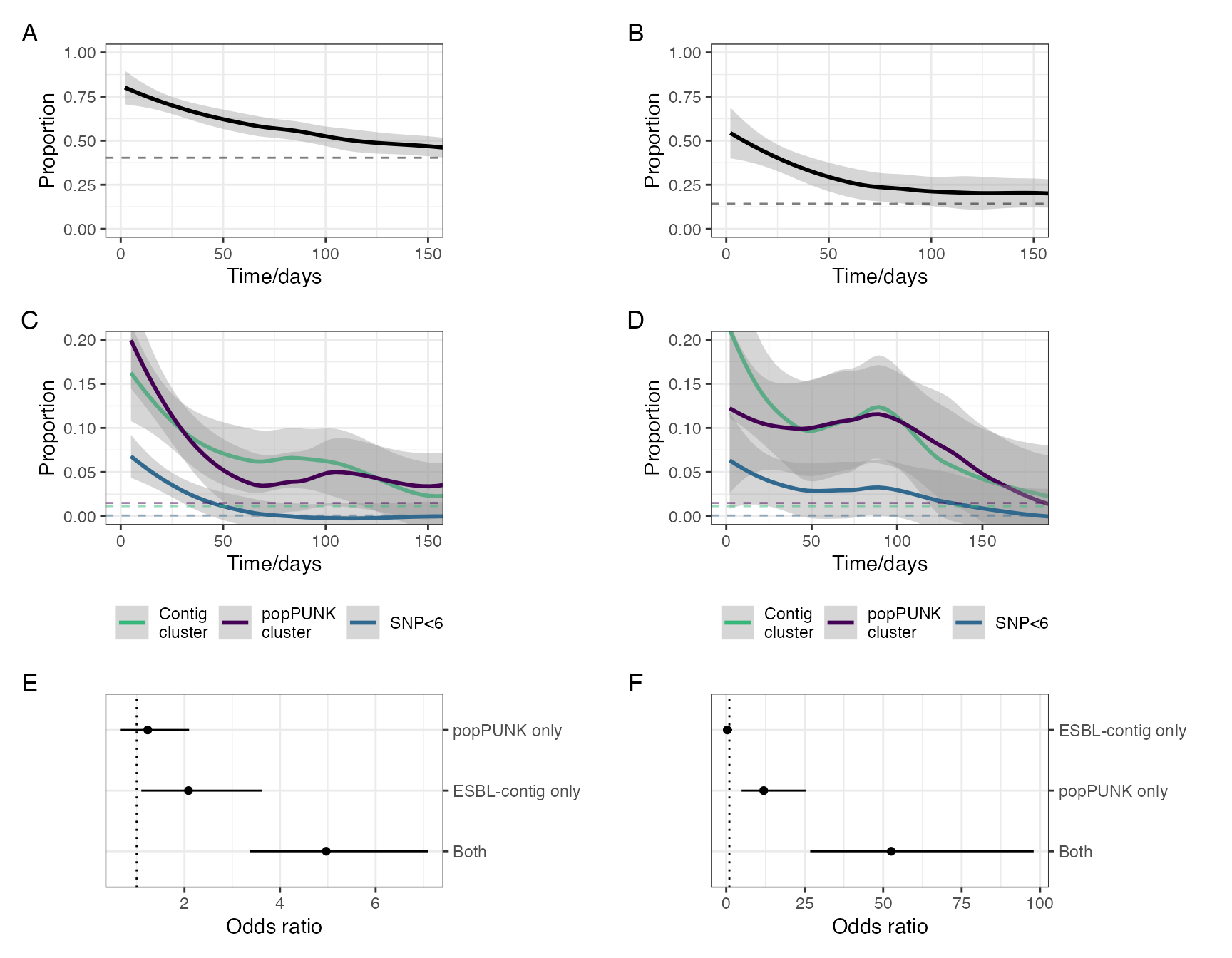
Within participant correlation of organism, lineage, mobile genetic element (MGE) and clone. A-B show proportions of participants that have a detectible E. coli (A), K. pneumoniae (B) at t time t=0 and the same organism at a time t later. Dashed lines show the proportion of samples in the collection that would be expected to have the same organism by chance: the proportion of between-participant samples that have the same organism. C shows (E. coli only) and D (for K. pneumoniae complex) the proportion of participants who are colonised with at time t=0 and the proportion of those who have the same lineage (as defined by popPUNK cluster), clone (as defined by <6 SNPs), or mobile genetic element (defined by ESBl-contig cluster) detectible a at time t later. Dashed lined again show the between-participant proportion of samples that contain the same lineage, clone or MGE to show the chance of obtaining any result ny chance. Fitted lines are from a nonparametric LOESS fit with 95% confidence intervals. D shows odds ratios of any within-participant E. coli pair containing the same popPUNK cluster only, ESBL-contig cluster, or both, compared to between-participant pairs, and E the same data for K. pneumoniae. It is more likely that both lineage (popPUNK cluster) and MGE (ESBL-cluster) are conserved together than either seperately, suggesting that the lineage-MGE combination is the conserved unit within this system.
Hospital associations of lineages and MGE
Hospital associations of popPUNK and contig clusters
btESBL_sequence_sample_metadata %>%
  as.data.frame() -> clusts

rownames(clusts) <- clusts$lane

plotcols <- viridis_pal()(4)[1:3]
names(plotcols) <- c("in_hospital","recent_dc","community")
# c( "grey86", "black", "grey65")


ggtree(btESBL_coregene_tree_esco) %>%
  gheatmap(
    clusts["hosp_assoc"],
    width = 0.05,
    color = NA,
    font.size = 3,
    colnames = FALSE
   # colnames_angle = 90,
  #  colnames_position = "top",
  #  colnames_offset_y = 10,
  )  +
 # ylim(c(0,500)) +
  geom_hilight(node = 727, fill = "red") +
  scale_fill_manual(values = plotcols,
                    labels =
                      c("In hospital",
                        "Post-discharge",
                        "Community"),
                    na.translate = FALSE)  +
  theme(legend.title = element_blank()) -> hospassoc.tree.esco
#> Scale for y is already present.
#> Adding another scale for y, which will replace the existing scale.
#> Scale for fill is already present.
#> Adding another scale for fill, which will replace the existing scale.

ggtree(tree_subset(btESBL_coregene_tree_kleb, 210,
                           levels_back = 0)) %>%
  gheatmap(
    clusts["hosp_assoc"],
    width = 0.05,
    color = NA,
    font.size = 3,
    colnames = FALSE
  #  colnames_angle = 90,
  #  colnames_position = "top",
  #  colnames_offset_y = 10,
  )  +
  #ylim(c(0,220)) +
  scale_fill_manual(values = plotcols,
                    labels =
                      c("In hospital",
                        "Post-discharge",
                        "Community"),
                    na.translate = FALSE
                              )  +
  theme(legend.title = element_blank()) -> hospassoc.tree.kleb
#> Scale for y is already present.
#> Adding another scale for y, which will replace the existing scale.
#> Scale for fill is already present.
#> Adding another scale for fill, which will replace the existing scale.


clusts %>%
  ungroup() %>%
  mutate(
    total_in_hosp = sum(hosp_assoc == "in_hospital", na.rm = TRUE),
    total_not_in_hosp = sum(hosp_assoc != "in_hospital", na.rm = TRUE)
  ) %>%
  group_by(Cluster) %>%
  summarise(
    clust_in_hosp = sum(hosp_assoc == "in_hospital", na.rm = TRUE),
    clust_not_in_hosp = sum(hosp_assoc != "in_hospital", na.rm = TRUE),
    total_in_hosp = median(total_in_hosp) - clust_in_hosp,
    total_not_in_hosp = median(total_not_in_hosp) - clust_not_in_hosp,
    pval = fisher.test(matrix(
      c(clust_in_hosp, total_in_hosp, clust_not_in_hosp, total_not_in_hosp), nrow = 2
    ), simulate.p.value = TRUE)$p.value
  ) %>%
  rename(clustr = Cluster) %>%
  mutate(log_pval = -log10(pval)) -> df.manhattan.popPUNK

ggplot(df.manhattan.popPUNK, aes(clustr, log_pval, color = log_pval >
                                   -log10(0.05 /
                                     nrow(df.manhattan.popPUNK)))) +
  geom_point(size = 0.5) +
  geom_hline(aes(yintercept = -log10(0.05 /
                                     nrow(df.manhattan.popPUNK))),
             linetype = "dashed") +
  theme_bw() +
  theme(
    legend.position = "none",
    axis.text.x = element_blank()) +
      scale_color_manual(values = c("black", "red")) +
  labs(y = "-log(p)", x = "popPUNK cluster") +
  geom_segment(aes(x = (23*1.3), y =  (3.66722 - 3.66722/3),
                   xend = 23 + 23*0.3*0.1, yend = 3.66722 - 0.1*3.66722/3),
               arrow = arrow(length = unit(0.3, "cm"))) ->
  manhattanplot_popPUNK
 #

## -- esbl clusters

btESBL_contigclusters %>%
  left_join(btESBL_sequence_sample_metadata,
            by = c("lane" = "lane")
  ) %>%
  as.data.frame() -> clusts_esbl


clusts_esbl %>%
  ungroup() %>%
  mutate(
    total_in_hosp = sum(hosp_assoc == "in_hospital", na.rm = TRUE),
    total_not_in_hosp = sum(hosp_assoc != "in_hospital", na.rm = TRUE)
  ) %>%
  group_by(clstr_name) %>%
  summarise(
    clust_in_hosp = sum(hosp_assoc == "in_hospital", na.rm = TRUE),
    clust_not_in_hosp = sum(hosp_assoc != "in_hospital", na.rm = TRUE),
    total_in_hosp = median(total_in_hosp) - clust_in_hosp,
    total_not_in_hosp = median(total_not_in_hosp) - clust_not_in_hosp,
    pval = fisher.test(matrix(
      c(clust_in_hosp, total_in_hosp, clust_not_in_hosp, total_not_in_hosp), nrow = 2
    ), simulate.p.value = TRUE)$p.value
  ) %>%
  mutate(log_pval = -log10(pval)) -> df.manhattan.esbl

ggplot(df.manhattan.esbl, aes(clstr_name, log_pval, color = log_pval >
                                   -log10(0.05 /
                                     nrow(df.manhattan.popPUNK)))) +
  geom_point(size = 0.5) +
  geom_hline(aes(yintercept = -log10(0.05 /
                                     nrow(df.manhattan.popPUNK))),
             linetype = "dashed") +
  theme_bw() +
  theme(
    legend.position = "none",
    axis.text.x = element_blank()) +
      scale_color_manual(values = c("black", "red")) +
  labs(y = "-log(p)", x = "Contig cluster") +
  geom_segment(aes(x = (27*1.3), y =  (3.680 - 3.680/3),
                   xend = 27 + 27*0.3*0.1, yend = 3.680 - 0.1*3.680/3),
               arrow = arrow(length = unit(0.3, "cm")) ) ->
  manhattanplot_esbl
 #

(((hospassoc.tree.esco |
  hospassoc.tree.kleb))) /
  (manhattanplot_popPUNK /
  manhattanplot_esbl) +
  plot_annotation(tag_levels = "A") +
  plot_layout(heights = c(1.5,1),
              guides = "collect") -> hosp_assoc_lineages

hosp_assoc_lineages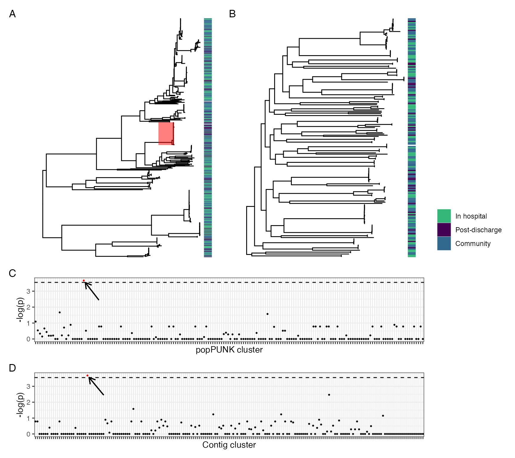
if (write_figs) {
  ggsave(here("figures/long-modelling/F4_hosp_assoc_lineages.pdf"),
         hosp_assoc_lineages,
         width = 9,
         height = 8)
  ggsave(here("figures/long-modelling/F4_hosp_assoc_lineages.svg"),
         hosp_assoc_lineages,
         width = 9,
         height = 8)
}
clusts %>%
  ungroup() %>%
  mutate(
    total_in_hosp = sum(hosp_assoc == "in_hospital" |
                          hosp_assoc == "recent_dc", na.rm = TRUE),
    total_not_in_hosp = sum(hosp_assoc == "community", na.rm = TRUE)
  ) %>%
  group_by(Cluster) %>%
  summarise(
    clust_in_hosp = sum(hosp_assoc == "in_hospital" |
                          hosp_assoc == "recent_dc", na.rm = TRUE),
    clust_not_in_hosp = sum(hosp_assoc == "community", na.rm = TRUE),
    total_in_hosp = median(total_in_hosp) - clust_in_hosp,
    total_not_in_hosp = median(total_not_in_hosp) - clust_not_in_hosp,
    pval = fisher.test(matrix(
      c(clust_in_hosp, total_in_hosp, clust_not_in_hosp, total_not_in_hosp), nrow = 2
    ), simulate.p.value = TRUE)$p.value
  ) %>%
  rename(clustr = Cluster) %>%
  mutate(log_pval = -log10(pval)) -> df.manhattan.popPUNK_sens

ggplot(df.manhattan.popPUNK_sens, aes(clustr, log_pval, color = log_pval >
                                   -log10(0.05 /
                                     nrow(df.manhattan.popPUNK_sens)))) +
  geom_point(size = 0.5) +
  geom_hline(aes(yintercept = -log10(0.05 /
                                     nrow(df.manhattan.popPUNK_sens))),
             linetype = "dashed") +
  theme_bw() +
  theme(
    legend.position = "none",
    axis.text.x = element_blank()) +
      scale_color_manual(values = c("black", "red")) +
  labs(y = "-log(p)", x = "popPUNK cluster") ->
  manhattanplot_popPUNK_sens

clusts_esbl %>%
  ungroup() %>%
  mutate(
    total_in_hosp = sum(hosp_assoc == "in_hospital" |
                          hosp_assoc == "recent_dc", na.rm = TRUE),
    total_not_in_hosp = sum(hosp_assoc == "community", na.rm = TRUE)
  ) %>%
  group_by(clstr_name) %>%
  summarise(
    clust_in_hosp = sum(hosp_assoc == "in_hospital" |
                          hosp_assoc == "recent_dc", na.rm = TRUE),
    clust_not_in_hosp = sum(hosp_assoc == "community", na.rm = TRUE),
    total_in_hosp = median(total_in_hosp) - clust_in_hosp,
    total_not_in_hosp = median(total_not_in_hosp) - clust_not_in_hosp,
    pval = fisher.test(matrix(
      c(clust_in_hosp, total_in_hosp, clust_not_in_hosp, total_not_in_hosp), nrow = 2
    ), simulate.p.value = TRUE)$p.value
  ) %>%
  mutate(log_pval = -log10(pval)) -> df.manhattan.esbl_sens

ggplot(df.manhattan.esbl_sens, aes(clstr_name, log_pval, color = log_pval >
                                   -log10(0.05 /
                                     nrow(df.manhattan.popPUNK)))) +
  geom_point(size = 0.5) +
  geom_hline(aes(yintercept = -log10(0.05 /
                                     nrow(df.manhattan.popPUNK))),
             linetype = "dashed") +
  theme_bw() +
  theme(
    legend.position = "none",
    axis.text.x = element_blank()) +
      scale_color_manual(values = c("black", "red")) +
  labs(y = "-log(p)", x = "Contig cluster") ->
  manhattanplot_esbl_sens

(manhattanplot_popPUNK_sens /
manhattanplot_esbl_sens) + plot_annotation(tag_levels = "A") ->
  hosp_assoc_lineages_sens


if (write_figs) {
  ggsave(here("figures/long-modelling/SUP_F_hosp_assoc_lineages.pdf"),
         hosp_assoc_lineages_sens,
         width = 9,
         height = 4)
  ggsave(here("figures/long-modelling/SUP_F_hosp_assoc_lineages.svg"),
         hosp_assoc_lineages_sens,
         width = 9,
         height = 4 )
}
Hospital association of SNP clusters
First, construct SNP clusters.
make_cluster_pairwise_comparison_df <- function(pairwise_snp_df,
                                                metadata_df,
                                                cut_tree_vect,
                                                n) {
  cluster_samples <- names(cut_tree_vect[cut_tree_vect == n])
  pairwise_snp_df <- as.data.frame(pairwise_snp_df)
  rownames(pairwise_snp_df) <- pairwise_snp_df$sample
  pairwise_snp_df[cluster_samples, c("sample", cluster_samples)] %>%
    pivot_longer(-sample) %>%
    filter(sample != name) -> d

  d[!duplicated(apply(d[1:2], 1, sort), MARGIN = 2), ] -> d
  names(d) <- c("sample.x", "sample.y", "snpdist")
  d$sample.x <- gsub("#", "_", d$sample.x)
  d$sample.y <- gsub("#", "_", d$sample.y)


  left_join(
    d,
    select(
      metadata_df,
      lane,
      pid,
      arm,
      visit,
      enroll_date,
      hospoutcomedate,
      data_date
    ),
    by = c("sample.x" = "lane")
  ) %>%
    left_join(
      select(
        metadata_df,
        lane,
        pid,
        arm,
        visit,
        enroll_date,
        hospoutcomedate,
        data_date
      ),
      by = c("sample.y" = "lane")
    ) -> d
  d$pair <- paste0(d$sample.x, "-", d$sample.y)
  d$cluster_number <- n
  d$cluster_name <- n
  d %>%
    mutate(type = case_when(pid.x == pid.y ~ "within",
                            TRUE ~ "between")) ->   d
  return(d)

}


make_all_clusters_pairwise_comparison_df  <-
  function(pairwise_snp_df,
           metadata_df,
           cut_tree_vect) {
    out <- list()
    for (i in 1:max(cut_tree_vect)) {
  #    print(i)
      #  print(i)
      make_cluster_pairwise_comparison_df(pairwise_snp_df,
                                          metadata_df,
                                          cut_tree_vect,
                                          i) -> out[[i]]

    }
    return(do.call(rbind, out))


  }


hclust(as.dist(btESBL_snpdists_esco[-1])) -> hclust_snpdists.e
cutree(hclust_snpdists.e, h = 5) -> cut_tree_vect.e

hclust(as.dist(btESBL_snpdists_kleb[-1])) -> hclust_snpdists.k
cutree(hclust_snpdists.k, h = 5) -> cut_tree_vect.k

as.data.frame(cut_tree_vect.e) %>%
  group_by(cut_tree_vect.e) %>%
  mutate(n = n()) %>%
  filter(n > 1) %>%
  ungroup() %>%
  summarise(med = median(n),
            lq = quantile(n, 0.25),
            uq = quantile(n, 0.75))
#> # A tibble: 1 × 3
#>     med    lq    uq
#>   <int> <dbl> <dbl>
#> 1     2     2     5

as.data.frame(cut_tree_vect.k) %>%
  group_by(cut_tree_vect.k) %>%
  mutate(n = n()) %>%
  filter(n > 1) %>%
  ungroup() %>%
  summarise(med = median(n),
            lq = quantile(n, 0.25),
            uq = quantile(n, 0.75))
#> # A tibble: 1 × 3
#>     med    lq    uq
#>   <int> <dbl> <dbl>
#> 1     2     2     3

make_all_clusters_pairwise_comparison_df(
  btESBL_snpdists_esco,
  btESBL_sequence_sample_metadata,
  cut_tree_vect.e) -> pairwise_snpclust.e


bind_rows(
  btESBL_sequence_sample_metadata %>%
    semi_join(btESBL_snpdists_esco,
              by = c("lane" = "sample")
    ) %>%
    select(lane, pid) %>%
    full_join(select(btESBL_sequence_sample_metadata, lane, pid) %>%
                semi_join(btESBL_snpdists_esco ,
                          by = c("lane" = "sample")),
              by = character())  %>%
    filter(lane.x != lane.y,
           pid.x == pid.y) %>%
    select(lane.x, lane.y) %>%
    mutate(type = "Same Patient") %>%
    rename(from = lane.x,
           to = lane.y),
  pairwise_snpclust.e %>%
    select(sample.x, sample.y) %>%
    rename(from = sample.x,
           to = sample.y) %>%
    mutate(type = "SNPs <6")

) -> edges.e


  btESBL_sequence_sample_metadata %>%
  semi_join(btESBL_snpdists_esco,
            by = c("lane" = "sample")
  ) %>%
  group_by(lane) %>%
  slice(1) %>%
    filter(!is.na(hosp_assoc)) %>%
  mutate(
    hosp_assoc = case_when(
      hosp_assoc == "community" ~ "Community",
      hosp_assoc == "in_hospital" ~ "In hospital",
      hosp_assoc == "recent_dc" ~ "Post discharge"),
    ) %>%
    relocate(lane, .before = everything()) ->
    vertices.e

edges.e %>%
  mutate(sortvar = map2_chr(from, to, ~paste(sort(c(.x,.y)), collapse = ""))) %>%
  group_by(sortvar,type) %>%
  slice(1) %>%
  ungroup() %>%
  select(-sortvar) %>%
  group_by(from,to) %>%
  mutate(weight = n()/10) %>%
  # remove those with missing metadata
  anti_join(
    btESBL_sequence_sample_metadata %>%
      filter(is.na(hosp_assoc)),
             by = c("from" = "lane")
      ) %>%
  anti_join(
    btESBL_sequence_sample_metadata %>%
      filter(is.na(hosp_assoc)),
             by = c("to" = "lane")
      ) -> edges.e


gr.e <- graph_from_data_frame(edges.e, directed = FALSE, vertices = vertices.e)

ggraph(gr.e, layout = "fr") +
  geom_edge_fan(aes(color = type), width = 1) +
  geom_node_point(aes(fill = hosp_assoc), shape = 21, size = 3) +
  #  facet_edges(~ type) +
  theme_void() + scale_fill_manual(values = c("white","black","grey")) +
  theme(legend.title = element_blank(), legend.position = "bottom",
        legend.text = element_text(size = 16)) +
  guides(edge_colour=guide_legend(ncol=1),
         fill=guide_legend(ncol=1)) ->
  snp_network_plot.esco

# kleb

make_all_clusters_pairwise_comparison_df(
  btESBL_snpdists_kleb,
  btESBL_sequence_sample_metadata,
  cut_tree_vect.k) -> pairwise_snpclust.k


bind_rows(
  btESBL_sequence_sample_metadata %>%
    semi_join(btESBL_snpdists_kleb,
              by = c("lane" = "sample")
    ) %>%
    select(lane, pid) %>%
    full_join(select(btESBL_sequence_sample_metadata, lane, pid) %>%
                semi_join(btESBL_snpdists_kleb ,
                          by = c("lane" = "sample")),
              by = character())  %>%
    filter(lane.x != lane.y,
           pid.x == pid.y) %>%
    select(lane.x, lane.y) %>%
    mutate(type = "Same Patient") %>%
    rename(from = lane.x,
           to = lane.y),
  pairwise_snpclust.k %>%
    select(sample.x, sample.y) %>%
    rename(from = sample.x,
           to = sample.y) %>%
    mutate(type = "SNPs <6")

) -> edges.k


  btESBL_sequence_sample_metadata %>%
  semi_join(btESBL_snpdists_kleb,
            by = c("lane" = "sample")
  ) %>%
  group_by(lane) %>%
  slice(1) %>%
    filter(!is.na(hosp_assoc)) %>%
  mutate(
    hosp_assoc = case_when(
      hosp_assoc == "community" ~ "Community",
      hosp_assoc == "in_hospital" ~ "In hospital",
      hosp_assoc == "recent_dc" ~ "Post discharge"),
    ) %>%
    relocate(lane, .before = everything()) ->
    vertices.k

edges.k %>%
  mutate(sortvar = map2_chr(from, to, ~paste(sort(c(.x,.y)), collapse = ""))) %>%
  group_by(sortvar,type) %>%
  slice(1) %>%
  ungroup() %>%
  select(-sortvar) %>%
  group_by(from,to) %>%
  mutate(weight = n()/10) %>%
  # remove those with missing metadata
  semi_join(
    vertices.k,
    by = c("from" = "lane")
      ) %>%
  semi_join(
    vertices.k, by = c("to" = "lane")
      ) -> edges.k


gr.k <- graph_from_data_frame(edges.k, directed = FALSE, vertices = vertices.k)

ggraph(gr.k, layout = "fr") + geom_edge_fan(aes(color = type), width = 1) +
  geom_node_point(aes(fill = hosp_assoc), shape = 21, size = 3) +
  #  facet_edges(~ type) +
  theme_void() + scale_fill_manual(values = c("white", "black", "grey")) +
  theme(
    legend.title = element_blank(),
    legend.position = "bottom",
    legend.text = element_text(size = 16)
  ) +
  guides(edge_colour = guide_legend(ncol = 1),
         fill = guide_legend(ncol = 1))  ->
  snp_network_plot.kleb


(snp_network_plot.esco +
  snp_network_plot.kleb) + plot_layout(guides = "collect") +
  plot_annotation(tag_levels = "A") &
  theme(legend.position = 'bottom',
        plot.tag = element_text(size = 22)) ->
  snp_networks
snp_networks
#> Warning: Using the `size` aesthetic in this geom was deprecated in ggplot2 3.4.0.
#> ℹ Please use `linewidth` in the `default_aes` field and elsewhere instead.
#> This warning is displayed once every 8 hours.
#> Call `lifecycle::last_lifecycle_warnings()` to see where this warning was
#> generated.![Network plot of SNP-clusters (i.e. putative transmission clusters) for E. coli (A) and K. pneumoniae (B) showing that putative transmission clusters are not purely hospital associated. Points are samples, coloured by place of isolation (in-hospital [black], community [white], or up to 120 days post-discharge [grey]). Red lines link samples that are within a single participant. Blue lines link samples that are differ by five or fewer SNPs. The plot shows that most samples are not members of a SNP-cluster; that most SNP clusters are made up of samples from different participants (rather than multiple samples from the same participant); and that SNP-clusters are not strongly hospital-associated (i.e. they contain black, white, and grey points).](analysis_files/figure-html/snp-clusts-1.png)
Network plot of SNP-clusters (i.e. putative transmission clusters) for E. coli (A) and K. pneumoniae (B) showing that putative transmission clusters are not purely hospital associated. Points are samples, coloured by place of isolation (in-hospital [black], community [white], or up to 120 days post-discharge [grey]). Red lines link samples that are within a single participant. Blue lines link samples that are differ by five or fewer SNPs. The plot shows that most samples are not members of a SNP-cluster; that most SNP clusters are made up of samples from different participants (rather than multiple samples from the same participant); and that SNP-clusters are not strongly hospital-associated (i.e. they contain black, white, and grey points).
Misc SNP cluster stats
## calculate stats about snpclusts
# how many in snp clusters are within vs between?
table(pairwise_snpclust.e$pid.x == pairwise_snpclust.e$pid.y)
#>
#> FALSE TRUE
#> 165 10
table(pairwise_snpclust.k$pid.x == pairwise_snpclust.k$pid.y)
#>
#> FALSE TRUE
#> 5 7
# what prop of clustered isolates are community vs hosp
btESBL_sequence_sample_metadata %>%
mutate(species = case_when(
lane %in% btESBL_coregene_tree_esco$tip.label ~ "esco",
lane %in% btESBL_coregene_tree_kleb$tip.label ~ "kleb"
)) %>%
semi_join(
bind_rows(
data.frame(lane = names(cut_tree_vect.e),
clust_name = cut_tree_vect.e) %>%
group_by(clust_name) %>%
mutate(n = n()) %>%
filter(n > 1),
data.frame(lane = names(cut_tree_vect.k),
clust_name = cut_tree_vect.k) %>%
group_by(clust_name) %>%
mutate(n = n()) %>%
filter(n > 1)
),
by = "lane"
) %>%
group_by(species, hosp_assoc) %>%
tally() %>%
pivot_wider(id_cols = species,
names_from = hosp_assoc,
values_from = n)
#> # A tibble: 2 × 5
#> # Groups: species [2]
#> species community in_hospital recent_dc `NA`
#> <chr> <int> <int> <int> <int>
#> 1 esco 54 19 77 1
#> 2 kleb 4 7 10 NA
# and for non SNP-clustered
btESBL_sequence_sample_metadata %>%
mutate(species = case_when(
lane %in% btESBL_coregene_tree_esco$tip.label ~ "esco",
lane %in% btESBL_coregene_tree_kleb$tip.label ~ "kleb"
)) %>%
semi_join(
bind_rows(
data.frame(lane = names(cut_tree_vect.e),
clust_name = cut_tree_vect.e) %>%
group_by(clust_name) %>%
mutate(n = n()) %>%
filter(n == 1),
data.frame(lane = names(cut_tree_vect.k),
clust_name = cut_tree_vect.k) %>%
group_by(clust_name) %>%
mutate(n = n()) %>%
filter(n == 1)
),
by = "lane"
) %>%
group_by(species, hosp_assoc) %>%
tally() %>%
pivot_wider(id_cols = species,
names_from = hosp_assoc,
values_from = n)
#> # A tibble: 2 × 5
#> # Groups: species [2]
#> species community in_hospital recent_dc `NA`
#> <chr> <int> <int> <int> <int>
#> 1 esco 117 59 145 1
#> 2 kleb 70 26 85 1
# What proportion of community isolates are members of SNP cluster
# vs in-hospital
btESBL_sequence_sample_metadata %>%
mutate(species = case_when(
lane %in% btESBL_coregene_tree_esco$tip.label ~ "esco",
lane %in% btESBL_coregene_tree_kleb$tip.label ~ "kleb"
)) %>%
left_join(
bind_rows(
data.frame(lane = names(cut_tree_vect.e),
clust_name = cut_tree_vect.e) %>%
group_by(clust_name) %>%
mutate(snp_clust_member = if_else(
n() > 1, "snp_clust_member",
"snp_clust_nonmember")),
data.frame(lane = names(cut_tree_vect.k),
clust_name = cut_tree_vect.k) %>%
group_by(clust_name) %>%
mutate(snp_clust_member = if_else(
n() > 1, "snp_clust_member",
"snp_clust_nonmember")),
),
by = "lane"
) %>%
mutate(hosp_assoc =
case_when(
grepl("hosp|_dc", hosp_assoc) ~ "healthcare_assoc",
TRUE ~ hosp_assoc)) %>%
group_by(species, hosp_assoc, snp_clust_member) %>%
tally() %>%
filter(!is.na(hosp_assoc)) %>%
group_by(species,hosp_assoc) %>%
mutate(total = sum(n)) %>%
filter(snp_clust_member == "snp_clust_member") %>%
select(-snp_clust_member) %>%
mutate(prop = n/total) %>%
group_by(species) %>%
nest() %>%
mutate(p = map(
data,
~ select(.x, -c(prop, hosp_assoc)) %>%
fisher.test(.x,simulate.p.value = TRUE) %>%
tidy() %>%
select(p.value))) %>%
unnest(cols = everything())
#> # A tibble: 4 × 6
#> # Groups: species [2]
#> species hosp_assoc n total prop p.value
#> <chr> <chr> <int> <int> <dbl> <dbl>
#> 1 esco community 54 171 0.316 1
#> 2 esco healthcare_assoc 96 300 0.32 1
#> 3 kleb community 4 74 0.0541 0.149
#> 4 kleb healthcare_assoc 17 128 0.133 0.149
# how many snp clusters contain 2 or more healthcare associated isolates?
btESBL_sequence_sample_metadata %>%
mutate(species = case_when(
lane %in% btESBL_coregene_tree_esco$tip.label ~ "esco",
lane %in% btESBL_coregene_tree_kleb$tip.label ~ "kleb"
)) %>%
left_join(
bind_rows(
data.frame(lane = names(cut_tree_vect.e),
snp_clust_name = paste0("E",cut_tree_vect.e)),
data.frame(lane = names(cut_tree_vect.k),
snp_clust_name = paste0("K",cut_tree_vect.k))
)) %>%
group_by(snp_clust_name) %>%
mutate(
healthcare_associated = case_when(
hosp_assoc == "community" ~ "Community",
hosp_assoc == "in_hospital" ~ "Healthcare associated",
hosp_assoc == "recent_dc" ~ "Healthcare associated",
TRUE ~ hosp_assoc),
snp_cluster_member = if_else(
n() > 1, "SNP cluster member", "SNP cluster nonmember")) %>%
group_by(snp_clust_name) %>%
mutate(
morethan1_cluster_member_hca =
case_when(
sum(healthcare_associated == "Healthcare associated",
na.rm = TRUE) > 1 ~ ">=2 HCA samples",
TRUE ~ "< 2 HCA samples")
) %>%
group_by(snp_cluster_member, morethan1_cluster_member_hca, species) %>%
filter(snp_cluster_member != "SNP cluster nonmember") %>%
group_by(snp_cluster_member, morethan1_cluster_member_hca, species) %>%
tally() %>%
group_by(species) %>%
mutate(tot = sum(n),
prop = n/tot) %>%
filter(grepl(">=", morethan1_cluster_member_hca)) %>%
group_by(species) %>%
mutate( lci = binom.test(n,tot)$conf.int[1],
uci = binom.test(n,tot)$conf.int[2])
#> Joining with `by = join_by(lane)`
#> # A tibble: 2 × 8
#> # Groups: species [2]
#> snp_cluster_member morethan1_cluster_member_…¹ species n tot prop lci
#> <chr> <chr> <chr> <int> <int> <dbl> <dbl>
#> 1 SNP cluster member >=2 HCA samples esco 98 151 0.649 0.567
#> 2 SNP cluster member >=2 HCA samples kleb 13 21 0.619 0.384
#> # ℹ abbreviated name: ¹morethan1_cluster_member_hca
#> # ℹ 1 more variable: uci <dbl>SNP cutoff sensitivity analysis
# sensitivity analysis of snp cutoffs

btESBL_snpdists_esco %>%
  pivot_longer(-sample) %>%
  rename("sample.x" = "sample",
         "sample.y" = "name",
         "snpdist_esco" = "value") %>%
  left_join(
    select(btESBL_sequence_sample_metadata, lane, supplier_name) %>%
      rename("lab_id.x" = "supplier_name"),
    by = c("sample.x" = "lane")) %>%
  left_join(
    select(btESBL_sequence_sample_metadata, lane, supplier_name) %>%
      rename("lab_id.y" = "supplier_name"),
    by = c("sample.y" = "lane")) %>%
  group_by(lab_id.x, lab_id.y) %>%
  slice(1) -> snpdist.e.long


btESBL_snpdists_kleb  %>%
  pivot_longer(-sample) %>%
  rename("sample.x" = "sample",
         "sample.y" = "name",
         "snpdist_kleb" = "value") %>%
  left_join(
    select(btESBL_sequence_sample_metadata, lane, supplier_name) %>%
      rename("lab_id.x" = "supplier_name"),
    by = c("sample.x" = "lane")) %>%
  left_join(
    select(btESBL_sequence_sample_metadata, lane, supplier_name) %>%
      rename("lab_id.y" = "supplier_name"),
    by = c("sample.y" = "lane")) %>%
  group_by(lab_id.x, lab_id.y) %>%
  slice(1)  -> snpdist.k.long

# make list-column df -----------------------------------------------------


btESBL_stoolESBL %>%
  left_join(btESBL_stoolorgs %>%
              filter(ESBL == "Positive") %>%
              select(lab_id, organism),
            by = "lab_id") %>%
  nest(orgs = organism) %>%
 left_join(
    select(btESBL_sequence_sample_metadata, supplier_name, Cluster),
    by = c("lab_id" = "supplier_name")
    ) %>%
  nest(pp_clust = Cluster) %>%
  left_join(
    btESBL_contigclusters %>%
      left_join(
        select(btESBL_sequence_sample_metadata , lane, supplier_name)
      ) %>%
      select(supplier_name, clstr_name),
    by = c("lab_id" = "supplier_name")
  ) %>%
  nest(contig_clust = clstr_name) %>%
  left_join(
    select(btESBL_sequence_sample_metadata, lane, supplier_name),
    by = c("lab_id" = "supplier_name")
  ) %>%
  nest(lanes = lane) -> samples
#> Joining with `by = join_by(lane)`

samples %>%
  full_join(samples, by = character())  %>%
  filter(lab_id.x != lab_id.y) %>%
  mutate(delta_t =
           interval(data_date.x, data_date.y) / days(1)) %>%
  filter(delta_t >= 0) -> samples
# compare presence absence of clusters

samples %>%
  mutate(esbl.x.and.y = ESBL.x == "Positive" &
           ESBL.y == "Positive") %>%
  #compare ESCO poppunk clusters between x and y
  # and add variables for e coli cluster and presence/absence
  # e coli to later remove isolates that weren't sequenced
  mutate(
    same.esco.poppunk.xandy =
      map2(pp_clust.x,
           pp_clust.y,
           ~ .x$Cluster[grepl("E", .x$Cluster)] %in%
             .y$Cluster[grepl("E", .y$Cluster)]) %>%
      map_lgl(any),
    # flags for existence of poppunk clusters
    esco.poppunk.cluster.exists.x =
      map(pp_clust.x, ~ grepl("E", .x$Cluster)) %>%
      map_lgl(any),
    esco.poppunk.cluster.exists.y =
      map(pp_clust.y, ~ grepl("E", .x$Cluster)) %>%
      map_lgl(any),
    # flag for existence of esco
    esco.exists.x =
      map_lgl(orgs.x, ~ any(grepl("coli", .x$organism))),
    esco.exists.y =
      map_lgl(orgs.y,  ~ any(grepl("coli", .x$organism))),
    same.esco.xandy = esco.exists.x & esco.exists.y,
    # contig clusters
    same.contig.cluster =
      map2(contig_clust.x,
           contig_clust.y,
           ~ .x$clstr_name %in%
             .y$clstr_name) %>%
      map_lgl(any)
  ) %>%
  # same but for klebs
  mutate(
    same.kleb.poppunk.xandy =
      map2(pp_clust.x,
           pp_clust.y,
           ~ .x$Cluster[grepl("K", .x$Cluster)] %in%
             .y$Cluster[grepl("K", .y$Cluster)]) %>%
      map_lgl(any),
    # flags for existence of poppunk clusters
    kleb.poppunk.cluster.exists.x =
      map(pp_clust.x, ~ grepl("K", .x$Cluster)) %>%
      map_lgl(any),
    kleb.poppunk.cluster.exists.y =
      map(pp_clust.y, ~ grepl("K", .x$Cluster)) %>%
      map_lgl(any),
    # flag for existence of kleb
    kleb.exists.x =
      map_lgl(orgs.x, ~ any(grepl("Klebsiella pneumoniae", .x$organism))),
    kleb.exists.y =
      map_lgl(orgs.y,  ~ any(grepl("Klebsiella pneumoniae", .x$organism))),
    same.kleb.xandy = kleb.exists.x & kleb.exists.y) ->
  samples

# merge in snpdist clusters

samples %>%
  left_join(
    select(snpdist.e.long, lab_id.x, lab_id.y, snpdist_esco),
    by = c("lab_id.x", "lab_id.y")
  ) %>%
  left_join(
    select(snpdist.k.long, lab_id.x, lab_id.y, snpdist_kleb),
    by = c("lab_id.x", "lab_id.y")
  ) -> samples

samples %>%
  filter(pid.x == pid.y) -> pairwise_within


pairwise_within %>%
  filter(esco.exists.x) %>%
  select(data_date.x, data_date.y,
         delta_t,
         esco.exists.x,
         esco.poppunk.cluster.exists.x,
         esco.exists.y,
         esco.poppunk.cluster.exists.y,
         delta_t,
         snpdist_esco) %>%
  pivot_longer(-c(data_date.x, data_date.y,
                  esco.exists.x, esco.exists.y,
                  esco.poppunk.cluster.exists.x,
                  esco.poppunk.cluster.exists.y,
                  delta_t)) %>%
  #filter out those with an esco but no poppunk cluster - they've not been
  # sequenced
  filter(
    !(esco.exists.x &
      !esco.poppunk.cluster.exists.x),
    !(esco.exists.y &
      !esco.poppunk.cluster.exists.y)
  ) -> ecoli.long

for (i in 0:20) {
  newcolvar <- paste0("snpdist_",i)
  ecoli.long %>%
    mutate({{newcolvar}} := if_else(
      value <= i & !is.na(value), TRUE, FALSE)
    ) -> ecoli.long
}

ecoli.long %>%
  select(delta_t, contains("snpdist")) %>%
  pivot_longer(-delta_t) %>%
  mutate(snpdist = as.numeric(gsub("snpdist_","", name))) %>%
  ggplot(aes(delta_t, as.numeric(value), color = snpdist, group = name)) +
    geom_smooth(se = FALSE) +
  scale_color_viridis_c() +
  coord_cartesian(xlim = c(0,150), ylim = c(0,0.13)) +
  theme_bw() +
  scale_y_continuous(breaks = c(0,0.02,0.04,0.06,0.08,0.1,0.12)) +
  labs(color = "SNP\ndistance",
       x = "Time/days",
       y = "Proportion") -> a


## klebs


pairwise_within %>%
  filter(kleb.exists.x) %>%
  select(data_date.x, data_date.y,
         delta_t,
         kleb.exists.x,
         kleb.poppunk.cluster.exists.x,
         kleb.exists.y,
         kleb.poppunk.cluster.exists.y,
         delta_t,
         snpdist_kleb) %>%
  pivot_longer(-c(data_date.x, data_date.y,
                  kleb.exists.x, kleb.exists.y,
                  kleb.poppunk.cluster.exists.x,
                  kleb.poppunk.cluster.exists.y,
                  delta_t)) %>%
  #filter out those with an kleb but no poppunk cluster - they've not been
  # sequenced
  filter(
    !(kleb.exists.x &
        !kleb.poppunk.cluster.exists.x),
    !(kleb.exists.y &
        !kleb.poppunk.cluster.exists.y)
  ) -> kleb.long

for (i in 0:20) {
  newcolvar <- paste0("snpdist_",i)
  kleb.long %>%
    mutate({{newcolvar}} := if_else(
      value <= i & !is.na(value), TRUE, FALSE)
    ) -> kleb.long
}

kleb.long %>%
  select(delta_t, contains("snpdist")) %>%
  pivot_longer(-delta_t) %>%
  mutate(snpdist = as.numeric(gsub("snpdist_","", name))) %>%
  ggplot(aes(delta_t, as.numeric(value), color = snpdist, group = name)) +
  geom_smooth(se = FALSE) +
  scale_color_viridis_c() +
  coord_cartesian(xlim = c(0,150),ylim = c(0,0.13)) +
  theme_bw() +
  scale_y_continuous(breaks = c(0,0.02,0.04,0.06,0.08,0.1,0.12)) +
  labs(color = "SNP\ndistance",
       x = "Time/days",
       y = "Proportion") -> b

a + b + plot_annotation(tag_levels = "A") +
plot_layout(guides = "collect") -> sens_analysis_within_snpdist

if (write_figs) {

  ggsave(here("figures/long-modelling/SUPP_FIG_sens_analysis_snpdist_autocorrelation.svg"),
         snp_networks,
         width = 9,
         height = 4)
  ggsave(here("figures/long-modelling/SUPP_FIG_sens_analysis_snpdist_autocorrelation.svg"),
         snp_networks,
         width = 9,
         height = 4)

}
#### start plots -------------

outlist.e.edges <- list()
outlist.e.vertices <- list()
outlist.e.plots <- list()
outlist.e.within_vs_betweendf <- list()

outlist.k.edges <- list()
outlist.k.vertices <- list()
outlist.k.plots <- list()
outlist.k.within_vs_betweendf <- list()

outlist.cluster_comm_vs_hosp <- list()

listindex <- 0

for (i in c(0,3,7,10)) {
  listindex = listindex + 1
  # make clusters for given snp dist
  hclust(as.dist(btESBL_snpdists_esco[-1])) -> hclust_snpdists.e
  cutree(hclust_snpdists.e, h = i) -> cut_tree_vect.e


  hclust(as.dist(btESBL_snpdists_kleb[-1])) -> hclust_snpdists.k
  cutree(hclust_snpdists.k, h = i) -> cut_tree_vect.k

  print(i)
  as.data.frame(cut_tree_vect.e) %>%
    group_by(cut_tree_vect.e) %>%
    mutate(n = n()) %>%
    filter(n > 1) %>%
    ungroup() %>%
    summarise(med = median(n),
              lq = quantile(n, 0.25),
              uq = quantile(n, 0.75))

  as.data.frame(cut_tree_vect.k) %>%
    group_by(cut_tree_vect.k) %>%
    mutate(n = n()) %>%
    filter(n > 1) %>%
    ungroup() %>%
    summarise(med = median(n),
              lq = quantile(n, 0.25),
              uq = quantile(n, 0.75))

  make_all_clusters_pairwise_comparison_df(btESBL_snpdists_esco,
                                           btESBL_sequence_sample_metadata,
                                           cut_tree_vect.e) -> pairwise_snpclust.e

  data.frame(
    "snp_dist" = i,
    "n_pairwise_snpclust_within" = sum(
      pairwise_snpclust.e$pid.x == pairwise_snpclust.e$pid.y,
      na.rm = TRUE
    ),
    "n_pairwise_snpclust_total" = nrow(pairwise_snpclust.e)
  ) -> within_vs_between_pairwise_df.e


  bind_rows(
    btESBL_sequence_sample_metadata %>%
      semi_join(btESBL_snpdists_esco,
                by = c("lane" = "sample")) %>%
      select(lane, pid) %>%
      full_join(
        select(btESBL_sequence_sample_metadata, lane, pid) %>%
          semi_join(btESBL_snpdists_esco ,
                    by = c("lane" = "sample")),
        by = character()
      )  %>%
      filter(lane.x != lane.y,
             pid.x == pid.y) %>%
      select(lane.x, lane.y) %>%
      mutate(type = "Same Patient") %>%
      rename(from = lane.x,
             to = lane.y),
    pairwise_snpclust.e %>%
      select(sample.x, sample.y) %>%
      rename(from = sample.x,
             to = sample.y) %>%
      mutate(type = "SNP cluster")

  ) -> edges.e


  btESBL_sequence_sample_metadata %>%
    semi_join(btESBL_snpdists_esco,
              by = c("lane" = "sample")) %>%
    group_by(lane) %>%
    slice(1) %>%
    filter(!is.na(hosp_assoc)) %>%
    mutate(
      hosp_assoc = case_when(
        hosp_assoc == "community" ~ "Community",
        hosp_assoc == "in_hospital" ~ "In hospital",
        hosp_assoc == "recent_dc" ~ "Post discharge"
      ),
    ) %>%
    relocate(lane, .before = everything()) ->
    vertices.e

  edges.e %>%
    mutate(sortvar = map2_chr(from, to, ~ paste(sort(c(
      .x, .y
    )), collapse = ""))) %>%
    group_by(sortvar, type) %>%
    slice(1) %>%
    ungroup() %>%
    select(-sortvar) %>%
    group_by(from, to) %>%
    mutate(weight = 0.1) %>%
    # remove those with missing metadata
    anti_join(btESBL_sequence_sample_metadata %>%
                filter(is.na(hosp_assoc)),
              by = c("from" = "lane")) %>%
    anti_join(btESBL_sequence_sample_metadata %>%
                filter(is.na(hosp_assoc)),
              by = c("to" = "lane")) -> edges.e


  gr.e <-
    graph_from_data_frame(edges.e, directed = FALSE, vertices = vertices.e)

  ggraph(gr.e, layout = "fr") + geom_edge_fan(aes(color = type), width =
                                                1) +
    geom_node_point(aes(fill = hosp_assoc), shape = 21, size = 3) +
    #  facet_edges(~ type) +
    theme_void() + scale_fill_manual(values = c("white", "black", "grey")) +
    theme(legend.title = element_blank()) ->
    snp_network_plot.esco

  outlist.e.edges[[listindex]] <- edges.e
  outlist.e.vertices[[listindex]] <- vertices.e
  outlist.e.plots[[listindex]] <- snp_network_plot.esco
  outlist.e.within_vs_betweendf[[listindex]] <-  within_vs_between_pairwise_df.e


  # kleb

  make_all_clusters_pairwise_comparison_df(btESBL_snpdists_kleb,
                                           btESBL_sequence_sample_metadata,
                                           cut_tree_vect.k) -> pairwise_snpclust.k

    data.frame(
    "snp_dist" = i,
    "n_pairwise_snpclust_within" = sum(
      pairwise_snpclust.k$pid.x == pairwise_snpclust.k$pid.y,
      na.rm = TRUE
    ),
    "n_pairwise_snpclust_total" = nrow(pairwise_snpclust.k)
  ) -> within_vs_between_pairwise_df.k

  bind_rows(
    btESBL_sequence_sample_metadata %>%
      semi_join(btESBL_snpdists_kleb,
                by = c("lane" = "sample")) %>%
      select(lane, pid) %>%
      full_join(
        select(btESBL_sequence_sample_metadata, lane, pid) %>%
          semi_join(btESBL_snpdists_kleb ,
                    by = c("lane" = "sample")),
        by = character()
      )  %>%
      filter(lane.x != lane.y,
             pid.x == pid.y) %>%
      select(lane.x, lane.y) %>%
      mutate(type = "Same Patient") %>%
      rename(from = lane.x,
             to = lane.y),
    pairwise_snpclust.k %>%
      select(sample.x, sample.y) %>%
      rename(from = sample.x,
             to = sample.y) %>%
      mutate(type = "SNP cluster")

  ) -> edges.k


  btESBL_sequence_sample_metadata %>%
    semi_join(btESBL_snpdists_kleb,
              by = c("lane" = "sample")) %>%
    group_by(lane) %>%
    slice(1) %>%
    filter(!is.na(hosp_assoc)) %>%
    mutate(
      hosp_assoc = case_when(
        hosp_assoc == "community" ~ "Community",
        hosp_assoc == "in_hospital" ~ "In hospital",
        hosp_assoc == "recent_dc" ~ "Post discharge"
      ),
    ) %>%
    relocate(lane, .before = everything()) ->
    vertices.k

  edges.k %>%
    mutate(sortvar = map2_chr(from, to, ~ paste(sort(c(
      .x, .y
    )), collapse = ""))) %>%
    group_by(sortvar, type) %>%
    slice(1) %>%
    ungroup() %>%
    select(-sortvar) %>%
    group_by(from, to) %>%
    mutate(weight = n() / 10) %>%
    # remove those with missing metadata
    semi_join(vertices.k,
              by = c("from" = "lane")) %>%
    semi_join(vertices.k, by = c("to" = "lane")) -> edges.k


  gr.k <-
    graph_from_data_frame(edges.k, directed = FALSE, vertices = vertices.k)

  ggraph(gr.k, layout = "fr") + geom_edge_fan(aes(color = type), width =
                                                1) +
    geom_node_point(aes(fill = hosp_assoc), shape = 21, size = 3) +
    #  facet_edges(~ type) +
    theme_void() + scale_fill_manual(values = c("white", "black", "grey")) +
    theme(legend.title = element_blank())  ->
    snp_network_plot.kleb

  outlist.k.edges[[listindex]] <- edges.k
  outlist.k.vertices[[listindex]] <- vertices.k
  outlist.k.plots[[listindex]] <- snp_network_plot.kleb
    outlist.k.within_vs_betweendf[[listindex]] <-  within_vs_between_pairwise_df.k


    # community vs not stats


btESBL_sequence_sample_metadata %>%
  mutate(species = case_when(
    lane %in% btESBL_coregene_tree_esco$tip.label  ~ "esco",
    lane %in% btESBL_coregene_tree_kleb$tip.label  ~ "kleb"
  )) %>%
  left_join(
    bind_rows(
      data.frame(lane = names(cut_tree_vect.e),
                 clust_name = cut_tree_vect.e) %>%
        group_by(clust_name) %>%
        mutate(cluster_member = if_else(n() > 1, "cluster_member", "cluster_nonmember")),
      data.frame(lane = names(cut_tree_vect.k),
                 clust_name = cut_tree_vect.k) %>%
        group_by(clust_name) %>%
        mutate(cluster_member = if_else(n() > 1, "cluster_member", "cluster_nonmember"))
    ),
    by = "lane"
  )  %>%
  mutate(cluster_member = as.factor(cluster_member)) %>%
  count(species, hosp_assoc, cluster_member, .drop = FALSE) %>%
  filter(!is.na(hosp_assoc)) %>%
  group_by(cluster_member, species) %>%
  mutate(total = sum(n),
         snp_dist = i) -> cluster_member_comm_assoc_df

outlist.cluster_comm_vs_hosp[[listindex]] <- cluster_member_comm_assoc_df

}
#> [1] 0
#> [1] 3
#> [1] 7
#> [1] 10

outlist.e.plots[[1]] +
  outlist.e.plots[[2]] +
  outlist.e.plots[[3]] +
  outlist.e.plots[[4]] +
  plot_layout(guides = "collect") +
  plot_annotation(tag_levels = "A") -> esco_snp_clusters_sens_analysis_plot

outlist.k.plots[[1]] +
  outlist.k.plots[[2]] +
  outlist.k.plots[[3]] +
  outlist.k.plots[[4]] +
  plot_layout(guides = "collect") +
  plot_annotation(tag_levels = "A") -> kleb_snp_clusters_sens_analysis_plot


esco_snp_clusters_sens_analysis_plot![Sensitivity analysis of network plot of putative transmission clusters for E. coli, allowing the definition of a SNP-cluster to vary from 0 (A), to 3 (B), 7 (C), or 10 (D). Points are samples, coloured by place of isolation (in-hospital [black], community [white], or up to 120 days post-discharge [grey]). Red lines link samples that are within a single participant. Blue lines link samples that are differ by the given SNP threshold.](analysis_files/figure-html/snp-network-sens-analysis-1.png)
Sensitivity analysis of network plot of putative transmission clusters for E. coli, allowing the definition of a SNP-cluster to vary from 0 (A), to 3 (B), 7 (C), or 10 (D). Points are samples, coloured by place of isolation (in-hospital [black], community [white], or up to 120 days post-discharge [grey]). Red lines link samples that are within a single participant. Blue lines link samples that are differ by the given SNP threshold.
if (write_figs) {
  ggsave(here("figures/long-modelling/SUPP_FIG_sens_analysis_snp_networks_esco.pdf"),
         esco_snp_clusters_sens_analysis_plot,
         width = 13.2,
         height = 12)
  ggsave(here("figures/long-modelling/SUPP_FIG_sens_analysis_snp_networks_esco.svg"),
         esco_snp_clusters_sens_analysis_plot,
         width = 13.2,
         height = 12)
}
kleb_snp_clusters_sens_analysis_plot![Sensitivity analysis of network plot of putative transmission clusters for E. coli, allowing the definition of a SNP-cluster to vary from 0 (A), to 3 (B), 7 (C), or 10 (D). Points are samples, coloured by place of isolation (in-hospital [black], community [white], or up to 120 days post-discharge [grey]). Red lines link samples that are within a single participant. Blue lines link samples that are differ by the given SNP threshold.](analysis_files/figure-html/snp-network-sens-analysis_kleb-1.png)
Sensitivity analysis of network plot of putative transmission clusters for E. coli, allowing the definition of a SNP-cluster to vary from 0 (A), to 3 (B), 7 (C), or 10 (D). Points are samples, coloured by place of isolation (in-hospital [black], community [white], or up to 120 days post-discharge [grey]). Red lines link samples that are within a single participant. Blue lines link samples that are differ by the given SNP threshold.
if (write_figs) {
  ggsave(here("figures/long-modelling/SUPP_FIG_sens_analysis_snp_networks_kleb.pdf"),
         kleb_snp_clusters_sens_analysis_plot,
         width = 13.2,
         height = 12)
  ggsave(here("figures/long-modelling/SUPP_FIG_sens_analysis_snp_networks_kleb.svg"),
         kleb_snp_clusters_sens_analysis_plot,
         width = 13.2,
         height = 12)
}
SNP cluster comparisons sensitivity analysis
bind_rows(
  do.call(bind_rows, outlist.k.within_vs_betweendf) %>%
    mutate(species = "K. pneumoniae"),
  do.call(bind_rows, outlist.e.within_vs_betweendf) %>%
    mutate(species = "E. coli")
) %>%
  rowwise() %>%
  mutate(
    prop = n_pairwise_snpclust_within/n_pairwise_snpclust_total,
    lci = binom.test(n_pairwise_snpclust_within,
                     n_pairwise_snpclust_total)$conf.int[[1]],
    uci = binom.test(n_pairwise_snpclust_within,
                     n_pairwise_snpclust_total)$conf.int[[2]]) -> within_vs_between

do.call(bind_rows,outlist.cluster_comm_vs_hosp ) %>%
  filter(hosp_assoc == "community") %>%
  rowwise() %>%
  mutate(
    prop = n/total,
    lci = binom.test(n,
                     total)$conf.int[[1]],
    uci = binom.test(n,
                     total)$conf.int[[2]]) -> comm_vs_hosp

within_vs_between %>%
  ggplot(aes(snp_dist, prop, ymin = lci, ymax = uci)) +
  geom_point() +
  geom_errorbar(width = 0) +
  facet_wrap(~ species) +
  theme_bw() +
  labs(y = "Proportion",
       x = "SNP distance") -> a

comm_vs_hosp %>%
  mutate(species =
           case_when(species == "esco" ~ "E. coli",
                     species == "kleb" ~ "K. pneumoniae"),
         cluster_member = gsub("_"," ",str_to_title(cluster_member))
         ) %>%
  ggplot(aes(snp_dist, prop, ymin = lci, ymax = uci, color = cluster_member, group = cluster_member))  +
           geom_point(position = position_dodge(width = 0.9)) +
  geom_errorbar(width = 0, position = position_dodge(width = 0.9)) +
  facet_wrap(~ species) +
  theme_bw() +
  labs(y = "Proportion",
       x = "SNP distance",
       color = "") -> b


outlist <- list()
listindex <- 0
for (i in c(0,3,7,10)) {
  listindex <- listindex + 1
  # make clusters for given snp dist
  hclust(as.dist(btESBL_snpdists_esco[-1])) -> hclust_snpdists.e
  cutree(hclust_snpdists.e, h = i) -> cut_tree_vect.e


  hclust(as.dist(btESBL_snpdists_kleb[-1])) -> hclust_snpdists.k
  cutree(hclust_snpdists.k, h = i) -> cut_tree_vect.k

btESBL_sequence_sample_metadata %>%
  mutate(species = case_when(
    lane %in% btESBL_coregene_tree_esco$tip.label  ~ "E. coli",
    lane %in% btESBL_coregene_tree_kleb$tip.label  ~ "K. pneumoniae"
  )) %>%
  left_join(
    bind_rows(
      data.frame(lane = names(cut_tree_vect.e),
                 snp_clust_name = paste0("E",cut_tree_vect.e)),
      data.frame(lane = names(cut_tree_vect.k),
                 snp_clust_name = paste0("K",cut_tree_vect.k))
    )) %>%
  group_by(snp_clust_name) %>%
  mutate(
    healthcare_associated = case_when(
      hosp_assoc == "community" ~ "Community",
      hosp_assoc == "in_hospital" ~ "Healthcare associated",
      hosp_assoc == "recent_dc" ~ "Healthcare associated",
      TRUE ~ hosp_assoc),
    snp_cluster_member = if_else(
      n() > 1, "SNP cluster member", "SNP cluster nonmember")) %>%
  group_by(snp_clust_name) %>%
  mutate(
    morethan1_cluster_member_hca =
      case_when(
        sum(healthcare_associated == "Healthcare associated",
            na.rm = TRUE) > 1 ~ ">=2 HCA samples",
        TRUE ~ "< 2 HCA samples")
  ) %>%
  group_by(snp_cluster_member, morethan1_cluster_member_hca, species) %>%
   tally()   %>%
  filter(snp_cluster_member != "SNP cluster nonmember") %>%
  group_by(species) %>%
  mutate(tot = sum(n),
         prop = n/tot) %>%
  filter(grepl(">=", morethan1_cluster_member_hca)) %>%
  group_by(species) %>%
  mutate( lci = binom.test(n,tot)$conf.int[1],
         uci = binom.test(n,tot)$conf.int[2],
         snp_cutoff = i) -> dfout
outlist[[listindex]] <- dfout
}
#> Joining with `by = join_by(lane)`
#> Joining with `by = join_by(lane)`
#> Joining with `by = join_by(lane)`
#> Joining with `by = join_by(lane)`

dfout <- do.call(rbind, outlist)

dfout %>%
ggplot(aes(snp_cutoff, prop, ymin = lci, ymax = uci)) +
  geom_point() +
  geom_errorbar(width = 0) +
  facet_wrap(~ species) +
  theme_bw() +
  labs(x = "SNP distance", y = "Proportion") -> c

(a / b / c) + plot_annotation(tag_levels = "A") -> sens.analysis.plot

#5 x 6.5
sens.analysis.plot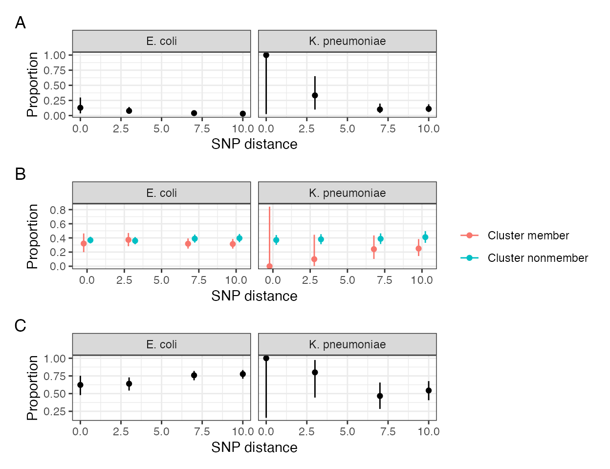
Sensitivity analysis examining epidemiology of SNP-clusters (i.e. putative transmission clusters) as the SNP-threshold varies from 0 to 10. (A) shows the proportion of pairwise comparisons of within-SNP-cluster isolates that are within a single participant; most putative transmission clusters are between-, rather than within- participants. (B) shows the proportion of isolates that are community associated stratified by whether they are members of a putative transmission cluster or not; the proportion is similar at all threshold values, which is not suggestive of hospital-associated transmission.
Reproducibility: packages used
sessionInfo()
#> R version 4.3.1 (2023-06-16)
#> Platform: aarch64-apple-darwin20 (64-bit)
#> Running under: macOS Sonoma 14.0
#>
#> Matrix products: default
#> BLAS:   /Library/Frameworks/R.framework/Versions/4.3-arm64/Resources/lib/libRblas.0.dylib
#> LAPACK: /Library/Frameworks/R.framework/Versions/4.3-arm64/Resources/lib/libRlapack.dylib;  LAPACK version 3.11.0
#>
#> locale:
#> [1] en_GB.UTF-8/en_GB.UTF-8/en_GB.UTF-8/C/en_GB.UTF-8/en_GB.UTF-8
#>
#> time zone: Europe/London
#> tzcode source: internal
#>
#> attached base packages:
#> [1] stats     graphics  grDevices utils     datasets  methods   base
#>
#> other attached packages:
#>  [1] blantyreESBL_1.4.1 kableExtra_1.3.4   ggtree_3.9.1       viridis_0.6.4
#>  [5] viridisLite_0.4.2  pheatmap_1.0.12    ggplotify_0.1.2    loo_2.6.0
#>  [9] patchwork_1.1.3    bayesplot_1.10.0   ggsci_3.0.0        broom_1.0.5
#> [13] glue_1.6.2         forcats_1.0.0      purrr_1.0.2        lubridate_1.9.3
#> [17] stringr_1.5.0      tidyr_1.3.0        dplyr_1.1.3        ggraph_2.1.0
#> [21] ggplot2_3.4.3      igraph_1.5.1       here_1.0.1         DescTools_0.99.50
#> [25] tidytree_0.4.5
#>
#> loaded via a namespace (and not attached):
#>   [1] RColorBrewer_1.1-3   tensorA_0.36.2       rstudioapi_0.15.0
#>   [4] jsonlite_1.8.7       magrittr_2.0.3       farver_2.1.1
#>   [7] rmarkdown_2.25       fs_1.6.3             ragg_1.2.5
#>  [10] vctrs_0.6.3          memoise_2.0.1        webshot_0.5.5
#>  [13] htmltools_0.5.6.1    distributional_0.3.2 cellranger_1.1.0
#>  [16] gridGraphics_0.5-1   sass_0.4.7           StanHeaders_2.26.28
#>  [19] bslib_0.5.1          desc_1.4.2           plyr_1.8.9
#>  [22] rootSolve_1.8.2.4    cachem_1.0.8         lifecycle_1.0.3
#>  [25] pkgconfig_2.0.3      Matrix_1.6-1.1       R6_2.5.1
#>  [28] fastmap_1.1.1        digest_0.6.33        Exact_3.2
#>  [31] aplot_0.2.2          colorspace_2.1-0     ps_1.7.5
#>  [34] rprojroot_2.0.3      textshaping_0.3.6    labeling_0.4.3
#>  [37] fansi_1.0.5          timechange_0.2.0     httr_1.4.7
#>  [40] polyclip_1.10-6      abind_1.4-5          mgcv_1.8-42
#>  [43] compiler_4.3.1       proxy_0.4-27         withr_2.5.1
#>  [46] backports_1.4.1      inline_0.3.19        QuickJSR_1.0.7
#>  [49] pkgbuild_1.4.2       highr_0.10           ggforce_0.4.1
#>  [52] MASS_7.3-60          gld_2.6.6            tools_4.3.1
#>  [55] ape_5.7-1            callr_3.7.3          nlme_3.1-162
#>  [58] grid_4.3.1           checkmate_2.2.0      reshape2_1.4.4
#>  [61] generics_0.1.3       gtable_0.3.4         class_7.3-22
#>  [64] data.table_1.14.8    lmom_3.0             tidygraph_1.2.3
#>  [67] xml2_1.3.5           utf8_1.2.3           ggrepel_0.9.3
#>  [70] pillar_1.9.0         yulab.utils_0.1.0    posterior_1.4.1
#>  [73] splines_4.3.1        tweenr_2.0.2         treeio_1.26.0
#>  [76] lattice_0.21-8       tidyselect_1.2.0     knitr_1.44
#>  [79] gridExtra_2.3        svglite_2.1.2        stats4_4.3.1
#>  [82] xfun_0.40            expm_0.999-7         graphlayouts_1.0.1
#>  [85] matrixStats_1.0.0    rstan_2.32.3         stringi_1.7.12
#>  [88] lazyeval_0.2.2       ggfun_0.1.3          yaml_2.3.7
#>  [91] boot_1.3-28.1        evaluate_0.22        codetools_0.2-19
#>  [94] tibble_3.2.1         cli_3.6.1            RcppParallel_5.1.7
#>  [97] systemfonts_1.0.4    munsell_0.5.0        processx_3.8.2
#> [100] jquerylib_0.1.4      Rcpp_1.0.11          readxl_1.4.3
#> [103] parallel_4.3.1       ellipsis_0.3.2       pkgdown_2.0.7
#> [106] prettyunits_1.2.0    mvtnorm_1.2-3        scales_1.2.1
#> [109] e1071_1.7-13         ggridges_0.5.4       crayon_1.5.2
#> [112] rlang_1.1.1          rvest_1.0.3