Longitudinal carriage: simulations to explore impact of one colony pick
simulations.RmdIntroduction and Methods
It is possible that one colony pick per time point could miss hospital acquisitions and hence miss hospital-associated clusters, due to a rapid flux of strains com-pared to intervals between sampling times. In this document we use a simulation approach to quantify how much of a problem this could be.
To set this up we assume:
- A population of \(N\) participant
- With each participant starting at time \(t=0\) colonised with a number \(n_{0}\) ESBL strains, where \(n_{0}\) is sampled from a Poisson distribution with rate \(\lambda\) (See Figure)
- A daily probability of loss of any ESBL strain of \(p_{loss}\)
- A daily probability of gain of any ESBL strain of \(p_{gain}\)
- That all ESBL strains (at \(t=0\) and any gains during the simulation period) are sampled from a population of 1000 with replacement and with equal probability of any strain being selected.
We can then simulate an outbreak by spiking the population with a hospital acquired strain at time 0 and ask - what is the probability of recovering this hospital acquired strain (\(p_{recovery}\)) by sampling a single colony pick at 7 (and hence identifying this sample as part of the “outbreak”)? We can run 10 simulations with say \(N=100\) participants and pool estimates with 95% CI to get a feel for how much of a problem it is.
In the above “strain” is deliberately vague - could consider it to be ST or a outbreak clone. IN fact in UK inpatients in Cambridge the within-ST diversity within-patient was limited (< 17 SNPs) so these could possible be considered the same thing (Ludden et al 2021)?
We then need to select some reasonable parameter values:
- Initial diversity; be guided by the literature; varying lambda between 1-5 seems reasonable (See Figure @ref(fig:plot-poisson))
- median 4 E. coli STs from 16 samples per participant in Cambodian infants (Stoesser et al 2015).
- mean 1-2 random amplified polymorphic DNA PCR (RAPD) patterns per participant in UK (Mosavie et al. 2019).
- UK adult inpatients: up to 15 colony picks at each time point 70% have 1 ST; 30% contain more than 1 (Ludden et al. 2021).
Probability of loss. Figure 2 in the manuscript suggests a return to baseline of probability of same-ST or SNP-cluster within participant over ~ 50 days. Hence \(p_{loss}\) = 0.05 per day seems reasonable which gives a half-life of 20 days.
Probability of acquisition. Given that this is a concern of the reviewer, lets vary this from 0 (no acquisition) to 0.2 per day in 0.05 steps
Then run the simulation forward a day at a time; calculate loss and gain using probabilities and sampling from a binomial distribution. On days that a “sample” is taken, randomly sample from all ESBL strains present in an individual.
library(dplyr)
library(ggplot2)
library(purrr)
library(here)

write_figs <- TRUE
if (write_figs) {
  if (!dir.exists(here("figures"))) {dir.create(here("figures"))}
  if (!dir.exists(here("tables"))) {dir.create(here("tables"))}

  if (!dir.exists(here("figures/long-modelling"))) {
    dir.create(here("figures/long-modelling"))
  }

  if (!dir.exists(here("tables/long-modelling"))) {
    dir.create(here("tables/long-modelling"))
    }
}
Results
tibble(
  n = rep(0:20,5),
  lambda = rep(1:5, each = 21)) %>%
  rowwise() %>%
  mutate(prob = dpois(n, lambda)) %>%
  ggplot(aes(n,prob, color = lambda, group = lambda)) +
  geom_line() +
  theme_bw() +
  scale_color_viridis_c() ->
  poissonplot

poissonplot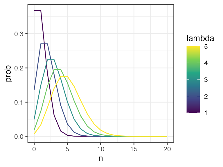
Poisson distribution with lambda varying from zero to five
if (write_figs) {
ggsave(here("figures/long-modelling/SUP_FIG_SIMSpoissonplot.pdf"), poissonplot,
      height = 3,
      width = 4
       )
ggsave(here("figures/long-modelling/SUP_FIG_SIMSpoissonplot.svg"), poissonplot,
      height = 3,
      width = 4
       )
}
# functions for sims

# updates an individual each day
update_states <- function(state_vector,
                          pr_gain,
                          pr_loss,
                          total_states) {
  # lose states
  if (length(state_vector) > 0) {
    state_vector <-
      state_vector[!as.logical(rbinom(length(state_vector), 1, pr_loss))]
  }
  # gain states
  if (rbinom(1, 1, pr_gain) == 1) {
    state_vector <- c(
      state_vector,
      sample(1:total_states, 1)
    )
  }
  if (length(state_vector) > 0) {
    return(state_vector)
  } else {
    return(vector(mode = "integer"))
  }
}

# sample from individuals strains
sample_states <- function(state_vector, strain) {
  if (length(state_vector > 0)) {
    sampl <- sample(state_vector, 1)
    return(strain == sampl)
  } else {
    return(FALSE)
  }
}
# walk through simulation for given parms and output dataframe

generate_sims <- function(nsims,
                          n_participants,
                          max_time,
                          pr_gain,
                          pr_loss,
                          n_start_states_median,
                          quiet = FALSE,
                          total_states = 1000) {
  simsout <- list()
  for (k in 1:nsims) {
    outlist <- list()
    for (j in 1:n_participants) {
      if (!quiet) {
        cat(
          paste0(
            "\r Replicate ", k, " of ", nsims,
            "  Participant ", j, " of ", n_participants,
            "     "
          )
        )
      }
      df <- tibble(
        rep = k,
        id = j,
        pid = rep(1, max_time + 1),
        t = 0:max_time,
        state_vector = c(
          list(c(1, sample(1:total_states, rpois(1, n_start_states_median)))),
          vector(mode = "list", length = max_time)
        ),
        pr_gain = rep(pr_gain, max_time + 1),
        pr_loss = rep(pr_loss, max_time + 1)
      )
      # populate states

      for (i in 2:nrow(df)) {
        # print(i)
        df$state_vector[[i]] <- update_states(df$state_vector[[i - 1]],
          df$pr_gain[i - 1],
          df$pr_loss[i - 1],
          total_states = total_states
        )
      }
      outlist[[j]] <- df
    }
    outdf <- do.call(rbind, outlist)
    simsout[[k]] <- outdf
  }
  simsdf <- do.call(rbind, simsout)
  return(simsdf)
}
# Now walk through parameter values
# vectors of parameter vals to iterate through
lambda_seq <- 0:5
pr_gain_seq <- c(0,0.05,0.1,0.15,0.2)

outlistouter <- list()
# total no of parameter combos
total <- length(pr_gain_seq)*length(lambda_seq)
counter <- 0

for (n in 1:length(pr_gain_seq)) {
  outlistinner <- list()
  for (m in 1:length(lambda_seq)) {
    counter <- counter + 1
    #cat("\rIteration ",counter, "/",total)
    generate_sims(
      nsims = 10,
      n_participants = 100,
      max_time = 100,
      pr_gain = pr_gain_seq[n],
      pr_loss = 0.05,
      n_start_states_median = lambda_seq[m],
      quiet = TRUE
    ) -> sim_df
    sim_df$lambda <- lambda_seq[m]
    outlistinner[[m]] <- sim_df
  }
  do.call(rbind, outlistinner) -> temp_df
  outlistouter[[n]] <- temp_df
}
do.call(rbind, outlistouter) -> simsall

pr_loss <- 0.05

# summarise to 95% CI ---------------------------------

simsall %>%
  mutate(
    sample_results = map_lgl(state_vector, ~ sample_states(.x, 1)),
    type = "samples",
    results = as.numeric(sample_results),
    results = if_else(t == 0, 1, results)
  ) %>%
  filter(t < 100, t > 0) %>%
  group_by(t, rep, lambda, pr_gain) %>%
  summarise(
    prop = sum(results) / length(results)
  ) %>%
  group_by(t, lambda, pr_gain) %>%
  summarise(
    prop_median = median(prop),
    lci = quantile(prop, 0.025),
    uci = quantile(prop, 0.975)
  ) -> sims_sum
sims_sum %>%
  mutate(type = "Simulation") %>%
  bind_rows(
    sims_sum %>%
      dplyr::select(t, lambda, pr_gain) %>%
      mutate(
        prop_median = (1 - pr_loss)^t,
        lci = NA,
        uci = NA,
        type = "True proportion"
      )
  ) %>%
  mutate(lambda = paste0("lambda ", lambda),
         pr_gain = paste0("pr_gain ", pr_gain)) %>%
  ggplot(aes(t, prop_median,
    ymin = lci, ymax = uci, fill = type,
    color = type
  )) +
  geom_line() +
  geom_ribbon(alpha = 0.3, color = NA) +
  facet_grid(pr_gain ~ lambda)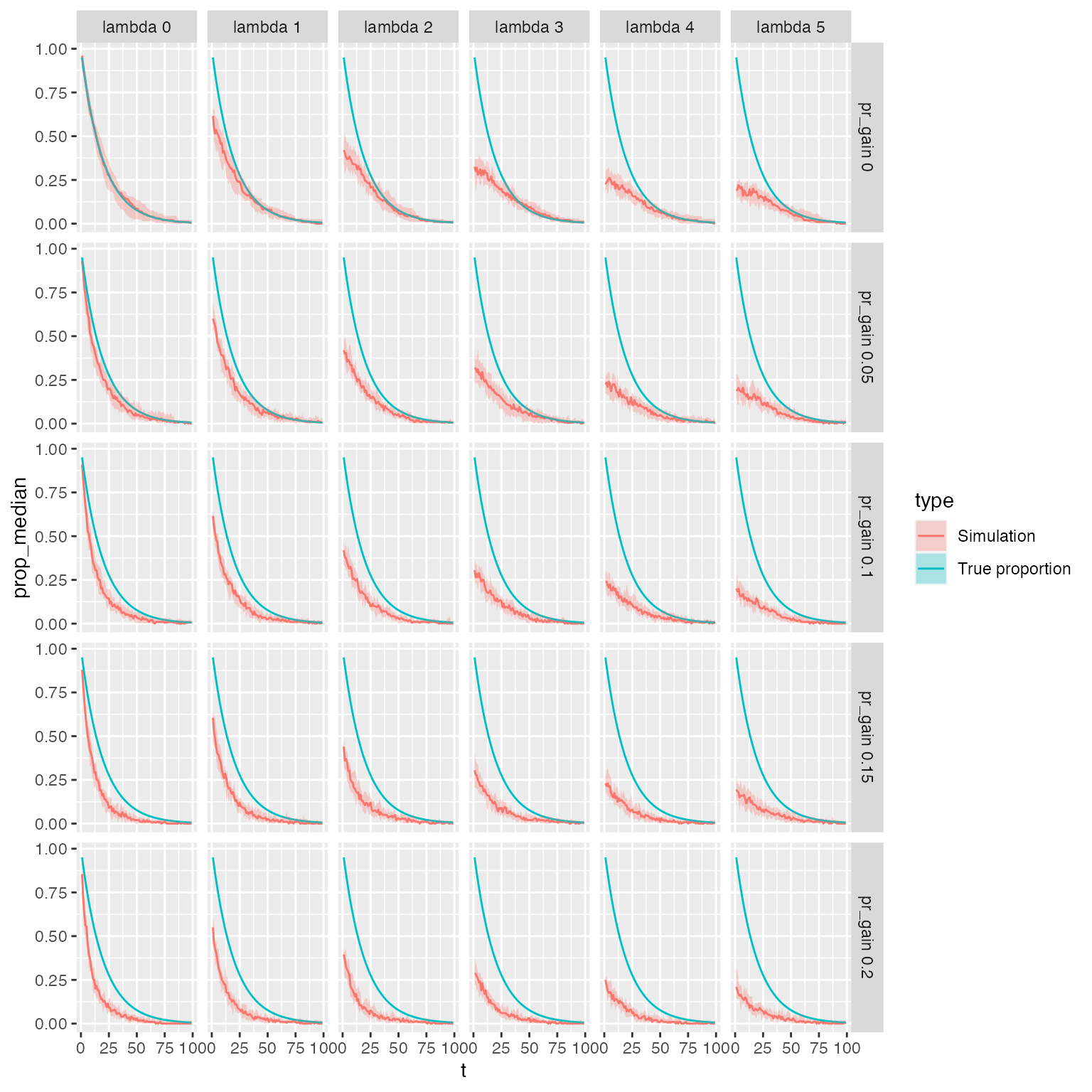
Assuming daily sampling, plots show the estimated proportion of samples (red line) that identify the hospital acquired ESBL strain that was present at time 0 given a single colony pick. Lambda (median number or carried ESBL strains) varies horizontally from 0 to 6; Daily probability of ESBL acquisition varies from 0 to 0.2 vertically. True proportion of samples that contain the hospital acquired strain shown by blue line..
sims_sum %>%
  filter(t %in% c(7)) %>%
  ggplot(aes(
    lambda,
    prop_median,
    ymin = lci,
    ymax = uci,
    color = pr_gain,
    fill = pr_gain,
    group = pr_gain
  )) +
  geom_point() +
  geom_line()  +
  geom_ribbon(alpha = 0.2, color = NA) +
  # facet_wrap(~ t) +
  ylim(c(0,0.8)) +
  labs(y = "Probability of identifying hospital strain" ) +
  theme_bw() ->
  simsprobplot

simsprobplot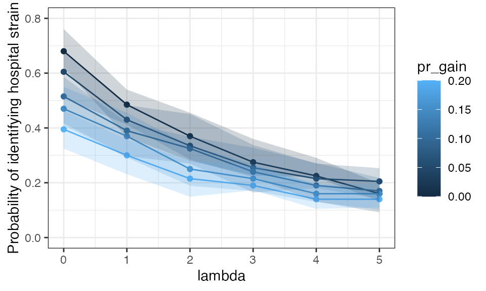
Probability of identifying strain present at day 0 on day 7 using a single colony pick as daily probability of acqusition of new strain (pr_gain) and initial strain diversity (defined by lambda) are varied.
Interpretation
So 27% (IQR 19-39%) of simulations across all parameter values recover the original strain and would identify the “outbreak”. Of course, this approach is an oversimplification: hospital associated strains could be acquired any time between t = 0 and t = 7; in this case, they would be more likely to be identified at day 7. Multiple circulating hospital strains, on the other hand would be less likely to be identified. Nevertheless, this simulation suggests that there is a reasonable chance of identifying a hospital outbreak.
References
Ludden, Catherine, Francesc Coll, Theodore Gouliouris, Olivier Restif, Beth Blane, Grace A Blackwell, Narender Kumar, et al. 2021. “Defining Nosocomial Transmission of Escherichia Coli and Antimicrobial Resistance Genes: A Genomic Surveillance Study.” The Lancet Microbe 2 (9): e472–80. https://doi.org/ 10.1016/S2666-5247(21)00117-8.
Mosavie, Mia, Oliver Blandy, Elita Jauneikaite, Isabel Caldas, Matthew J. Ellington, Neil Woodford, and Shiranee Sriskandan. 2019. “Sampling and Diversity of Escherichia Coli from the Enteric Microbiota in Patients with Escherichia Coli Bacteraemia.” BMC Research Notes 12 (1): 335. https://doi.org/10.1186/ s13104-019-4369-y.
Stoesser, N, A E Sheppard, C E Moore, T Golubchik, C M Parry, P Nget, M Saroeun, et al. 2015. “Extensive Within-Host Diversity in Fecally Carried Extended-Spectrum-Beta-Lactamase-Producing Escherichia Coli Isolates: Implications for Transmission Analyses.” Journal of Clinical Microbiology 53 (7): 212231. https://doi.org/10.1128/JCM.00378-15.