Analysis scripts: E. coli genomics
analysis-ecoli.RmdIntroduction
This document contains reproducing analysis code which generates the tables and figures for the manuscript:
Genomic analysis of extended-spectrum beta-lactamase (ESBL) producing Escherichia coli colonising adults in Blantyre, Malawi reveals previously undescribed diversity
Joseph M Lewis1,2,3,4, , Madalitso Mphasa1, Rachel Banda1, Matthew Beale4, Jane Mallewa5, Catherine Anscombe1,2, Allan Zuza1, Adam P Roberts2, Eva Heinz*2, Nicholas Thomson*4,6, Nicholas A Feasey*1,2
- Malawi Liverpool Wellcome Research Programme, Blantyre, Malawi
- Liverpool School of Tropical Medicine, Liverpool, UK
- University of Liverpool, Liverpool, UK
- Wellcome Sanger Institute, Hinxton, UK
- Kamuzu University of Health Sciences, Malawi
- London School of Tropical Medicine and Hygiene, London, UK
- = contributed equally
library(tidytree)
#> If you use the ggtree package suite in published research,
#> please cite the appropriate paper(s):
#>
#> LG Wang, TTY Lam, S Xu, Z Dai, L Zhou, T Feng, P Guo, CW Dunn, BR
#> Jones, T Bradley, H Zhu, Y Guan, Y Jiang, G Yu. treeio: an R package
#> for phylogenetic tree input and output with richly annotated and
#> associated data. Molecular Biology and Evolution. 2020, 37(2):599-603.
#> doi: 10.1093/molbev/msz240
#>
#> Guangchuang Yu.  Data Integration, Manipulation and Visualization of
#> Phylogenetic Trees (1st edition). Chapman and Hall/CRC. 2022,
#> doi:10.1201/9781003279242
#>
#> Attaching package: 'tidytree'
#> The following object is masked from 'package:stats':
#>
#>     filter
library(ggtree)
#> ggtree v3.9.1 For help: https://yulab-smu.top/treedata-book/
#>
#> If you use the ggtree package suite in published research, please cite
#> the appropriate paper(s):
#>
#> Guangchuang Yu, David Smith, Huachen Zhu, Yi Guan, Tommy Tsan-Yuk Lam.
#> ggtree: an R package for visualization and annotation of phylogenetic
#> trees with their covariates and other associated data. Methods in
#> Ecology and Evolution. 2017, 8(1):28-36. doi:10.1111/2041-210X.12628
#>
#> G Yu. Data Integration, Manipulation and Visualization of Phylogenetic
#> Trees (1st ed.). Chapman and Hall/CRC. 2022. ISBN: 9781032233574
#>
#> Guangchuang Yu.  Data Integration, Manipulation and Visualization of
#> Phylogenetic Trees (1st edition). Chapman and Hall/CRC. 2022,
#> doi:10.1201/9781003279242
library(ape)
#>
#> Attaching package: 'ape'
#> The following object is masked from 'package:ggtree':
#>
#>     rotate
#> The following objects are masked from 'package:tidytree':
#>
#>     drop.tip, keep.tip
library(phytools)
#> Loading required package: maps
library(dplyr)
#>
#> Attaching package: 'dplyr'
#> The following object is masked from 'package:ape':
#>
#>     where
#> The following objects are masked from 'package:stats':
#>
#>     filter, lag
#> The following objects are masked from 'package:base':
#>
#>     intersect, setdiff, setequal, union
library(tidyr)
#>
#> Attaching package: 'tidyr'
#> The following object is masked from 'package:ggtree':
#>
#>     expand
library(readr)
library(ggplot2)
library(forcats)
library(stringr)
library(blantyreESBL)
library(lubridate)
#>
#> Attaching package: 'lubridate'
#> The following objects are masked from 'package:base':
#>
#>     date, intersect, setdiff, union
library(ggnewscale)
library(kableExtra)
#>
#> Attaching package: 'kableExtra'
#> The following object is masked from 'package:dplyr':
#>
#>     group_rows
library(patchwork)
library(here)
#> here() starts at /Users/joelewis/R/packages/blantyreESBL
library(scales)
#>
#> Attaching package: 'scales'
#> The following object is masked from 'package:readr':
#>
#>     col_factor
#> The following object is masked from 'package:phytools':
#>
#>     rescale
library(ggstance)
#>
#> Attaching package: 'ggstance'
#> The following objects are masked from 'package:ggplot2':
#>
#>     geom_errorbarh, GeomErrorbarh
library(blantyreESBL)
library(countrycode)
library(viridis)
#> Loading required package: viridisLite
#>
#> Attaching package: 'viridis'
#> The following object is masked from 'package:scales':
#>
#>     viridis_pal
#> The following object is masked from 'package:maps':
#>
#>     unemp

write_figs <- FALSE

if (write_figs) {
  if (!dir.exists(here("figures"))) {dir.create(here("figures"))}
  if (!dir.exists(here("tables"))) {dir.create(here("tables"))}

    if (!dir.exists(here("figures/ecoli-genomics"))) {
    dir.create(here("figures/ecoli-genomics"))
  }

  if (!dir.exists(here("tables/ecoli-genomics"))) {
    dir.create(here("tables/ecoli-genomics"))
    }

}
Assembly stats and accession numbers
btESBL_sequence_sample_metadata %>%
  mutate(date_of_collection = data_date) %>%
  select(accession,
         lane,
         supplier_name,
         pid,
         date_of_collection,
         N50) %>%
  kbl(caption =
        "Accession numbers and assembly statistics for included samples"
      ) %>%
kable_classic(full_width = FALSE)| accession | lane | supplier_name | pid | date_of_collection | N50 |
|---|---|---|---|---|---|
| ERR3425924 | 26141_1_134 | CAB153 | DAS10020 | 2017-09-13 | 90677 |
| ERR3425925 | 26141_1_135 | CAC127 | DAS10020 | 2017-09-20 | 91797 |
| ERR3425926 | 26141_1_136 | CAD13R | DAS10020 | 2017-10-12 | 90587 |
| ERR3425927 | 26141_1_137 | CAE12N | DAS10020 | 2017-12-13 | 214462 |
| ERR3425928 | 26141_1_138 | CAI10E | DAS1005V | 2017-10-10 | 132088 |
| ERR3425929 | 26141_1_139 | CAJ10A | DAS1005V | 2017-12-12 | 207354 |
| ERR3425930 | 26141_1_140 | CAD13P | DAS1006T | 2017-10-09 | 106469 |
| ERR3425931 | 26141_1_141 | CAI10F | DAS10100 | 2017-10-17 | 147795 |
| ERR3425932 | 26141_1_142 | CAB14X | DAS1014T | 2017-09-07 | 179790 |
| ERR3425933 | 26141_1_143 | CAC11I | DAS1014T | 2017-09-14 | 190526 |
| ERR3425934 | 26141_1_144 | CAD137 | DAS1014T | 2017-10-06 | 186956 |
| ERR3425935 | 26141_1_145 | CAE12R | DAS1014T | 2017-12-18 | 91797 |
| ERR3425936 | 26141_1_146 | CAL10S | DAS1016P | 2017-09-27 | 132400 |
| ERR3425937 | 26141_1_147 | CAM10R | DAS1016P | 2017-11-08 | 126233 |
| ERR3425938 | 26141_1_148 | CAM10K | DAS1019J | 2017-10-05 | 96590 |
| ERR3425939 | 26141_1_149 | CAC126 | DAS1020X | 2017-09-12 | 71986 |
| ERR3425940 | 26141_1_150 | CAB13C | DAS1024P | 2017-09-01 | 212649 |
| ERR3425941 | 26141_1_151 | CAC124 | DAS1024P | 2017-09-07 | 222532 |
| ERR3425942 | 26141_1_152 | CAD13N | DAS1024P | 2017-09-28 | 241104 |
| ERR3425943 | 26141_1_153 | CAE12K | DAS1024P | 2017-12-01 | 207364 |
| ERR3425944 | 26141_1_154 | CAC122 | DAS1028H | 2017-09-05 | 183579 |
| ERR3425945 | 26141_1_155 | CAE12H | DAS1028H | 2017-11-28 | 95953 |
| ERR3425946 | 26141_1_156 | CAB139 | DAS1029F | 2017-08-29 | 227316 |
| ERR3425947 | 26141_1_157 | CAC123 | DAS1029F | 2017-09-06 | 191270 |
| ERR3425948 | 26141_1_158 | CAD134 | DAS1029F | 2017-09-27 | 173030 |
| ERR3425949 | 26141_1_159 | CAE12L | DAS1029F | 2017-12-06 | 97192 |
| ERR3425950 | 26141_1_160 | CAD13K | DAS1034L | 2017-09-21 | 233352 |
| ERR3425951 | 26141_1_161 | CAE12F | DAS1035J | 2017-11-22 | 97056 |
| ERR3425952 | 26141_1_162 | CAC11X | DAS1042L | 2017-08-24 | 126528 |
| ERR3425954 | 26141_1_164 | CAB13L | DAS1047B | 2017-08-14 | 91797 |
| ERR3425955 | 26141_1_165 | CAC11F | DAS1047B | 2017-08-21 | 91797 |
| ERR3425956 | 26141_1_166 | CAD13J | DAS10489 | 2017-09-18 | 165340 |
| ERR3425958 | 26141_1_168 | CAM10H | DAS1053F | 2017-09-15 | 233363 |
| ERR3425959 | 26141_1_169 | CAB13I | DAS1055B | 2017-08-09 | 97260 |
| ERR3425960 | 26141_1_170 | CAD12Z | DAS1055B | 2017-09-01 | 173896 |
| ERR3425961 | 26141_1_171 | CAC11W | DAS10593 | 2017-08-10 | 191259 |
| ERR3425962 | 26141_1_172 | CAC11C | DAS1060H | 2017-08-08 | 222887 |
| ERR3425963 | 26141_1_173 | CAD115 | DAS1060H | 2017-08-30 | 222890 |
| ERR3425964 | 26141_1_174 | CAE110 | DAS1060H | 2017-11-01 | 239980 |
| ERR3425965 | 26141_1_175 | CAC119 | DAS10649 | 2017-08-07 | 404954 |
| ERR3425966 | 26141_1_176 | CAE10Z | DAS10649 | 2017-10-30 | 118863 |
| ERR3425967 | 26141_1_177 | CAB12F | DAS10657 | 2017-07-24 | 249398 |
| ERR3425968 | 26141_1_178 | CAC11D | DAS10657 | 2017-08-11 | 97316 |
| ERR3425969 | 26141_1_179 | CAD113 | DAS10657 | 2017-08-28 | 133224 |
| ERR3425970 | 26141_1_180 | CAE116 | DAS10657 | 2017-11-16 | 225549 |
| ERR3425971 | 26141_1_181 | CAH108 | DAS10673 | 2017-07-28 | 204492 |
| ERR3425972 | 26141_1_182 | CAI107 | DAS10673 | 2017-08-18 | 133224 |
| ERR3425973 | 26141_1_183 | CAJ105 | DAS10673 | 2017-10-24 | 126601 |
| ERR3425974 | 26141_1_184 | CAG10D | DAS1069X | 2017-07-20 | 154938 |
| ERR3425976 | 26141_1_186 | CAB12D | DAS1070D | 2017-07-19 | 192844 |
| ERR3425977 | 26141_1_187 | CAC116 | DAS10753 | 2017-07-20 | 132069 |
| ERR3425979 | 26141_1_189 | CAC117 | DAS1077X | 2017-07-24 | 210236 |
| ERR3425980 | 26141_1_190 | CAD10X | DAS1077X | 2017-08-14 | 201425 |
| ERR3425981 | 26141_1_191 | CAJ102 | DAS1079W | 2017-09-26 | 156945 |
| ERR3425982 | 26141_1_192 | CAG106 | DAS10841 | 2017-06-28 | 99469 |
| ERR3425983 | 26141_1_193 | CAH103 | DAS10841 | 2017-07-05 | 99469 |
| ERR3425984 | 26141_1_194 | CAI109 | DAS10841 | 2017-08-28 | 233352 |
| ERR3425985 | 26141_1_195 | CAJ109 | DAS10841 | 2017-12-06 | 106468 |
| ERR3425986 | 26141_1_196 | CAM107 | DAS1087W | 2017-07-13 | 209178 |
| ERR3425987 | 26141_1_197 | CAM10B | DAS1088U | 2017-08-11 | 233352 |
| ERR3425988 | 26141_1_198 | CAB11F | DAS10905 | 2017-06-13 | 221680 |
| ERR3425989 | 26141_1_199 | CAC10Y | DAS10905 | 2017-06-20 | 211377 |
| ERR3425990 | 26141_1_200 | CAE10Q | DAS10905 | 2017-09-26 | 211370 |
| ERR3425991 | 26141_1_201 | CAC110 | DAS10913 | 2017-06-28 | 204336 |
| ERR3425992 | 26141_1_202 | CAD10T | DAS10913 | 2017-07-18 | 248198 |
| ERR3425993 | 26141_1_203 | CAE10N | DAS10913 | 2017-09-20 | 106481 |
| ERR3425994 | 26141_1_204 | CAG10A | DAS10921 | 2017-07-06 | 91797 |
| ERR3425995 | 26141_1_205 | CAI104 | DAS10921 | 2017-08-04 | 91797 |
| ERR3425996 | 26141_1_206 | CAB11K | DAS1093X | 2017-06-29 | 206614 |
| ERR3425997 | 26141_1_207 | CAE10T | DAS1093X | 2017-10-06 | 131790 |
| ERR3425998 | 26141_1_208 | CAF10N | DAS1093X | 2017-12-22 | 82303 |
| ERR3425999 | 26141_1_209 | CAC111 | DAS1096U | 2017-06-29 | 241155 |
| ERR3426000 | 26141_1_210 | CAE10P | DAS1096U | 2017-09-22 | 201442 |
| ERR3426001 | 26141_1_211 | CAF10J | DAS1096U | 2017-12-04 | 214462 |
| ERR3426002 | 26141_1_212 | CAL108 | DAS1098Q | 2017-06-19 | 91797 |
| ERR3426003 | 26141_1_213 | CAM108 | DAS1098Q | 2017-07-17 | 147807 |
| ERR3426004 | 26141_1_214 | CAE10V | DAS1100X | 2017-10-18 | 99443 |
| ERR3426005 | 26141_1_215 | CAC10V | DAS1107J | 2017-06-05 | 407409 |
| ERR3426007 | 26141_1_217 | CAF10G | DAS1107J | 2017-11-17 | 209764 |
| ERR3426008 | 26141_1_218 | CAC10X | DAS1111R | 2017-06-20 | 129521 |
| ERR3426009 | 26141_1_219 | CAD10M | DAS1111R | 2017-07-04 | 210234 |
| ERR3426010 | 26141_1_220 | CAF10K | DAS1111R | 2017-12-06 | 73328 |
| ERR3426011 | 26141_1_221 | CAG104 | DAS1113N | 2017-06-09 | 97252 |
| ERR3426012 | 26141_1_222 | CAH101 | DAS1113N | 2017-06-16 | 101609 |
| ERR3426013 | 26141_1_223 | CAI101 | DAS1113N | 2017-07-11 | 101512 |
| ERR3426014 | 26141_1_224 | CAC10Z | DAS1116H | 2017-06-27 | 179783 |
| ERR3426015 | 26141_1_225 | CAD10Q | DAS1116H | 2017-07-17 | 132553 |
| ERR3426016 | 26141_1_226 | CAE10S | DAS1116H | 2017-09-27 | 97068 |
| ERR3426017 | 26141_1_227 | CAB11R | DAS1125F | 2017-05-03 | 213110 |
| ERR3426018 | 26141_1_228 | CAC10R | DAS1125F | 2017-05-09 | 212649 |
| ERR3426019 | 26141_1_229 | CAE10K | DAS1125F | 2017-08-24 | 132500 |
| ERR3426020 | 26141_1_230 | CAF10E | DAS1125F | 2017-11-17 | 185271 |
| ERR3426022 | 26141_1_232 | CAC10Q | DAS1126D | 2017-05-09 | 210215 |
| ERR3426026 | 26141_1_236 | CAC10S | DAS11289 | 2017-05-09 | 126680 |
| ERR3426027 | 26141_1_237 | CAL101 | DAS1130L | 2017-04-24 | 209880 |
| ERR3426029 | 26141_1_239 | CAM100 | DAS1133F | 2017-05-18 | 170302 |
| ERR3426030 | 26141_1_240 | CAD110 | DAS11369 | 2017-08-17 | 148760 |
| ERR3426031 | 26141_1_241 | CAE10W | DAS11369 | 2017-10-18 | 473927 |
| ERR3426032 | 26141_1_242 | CAI100 | DAS11377 | 2017-07-06 | 92256 |
| ERR3426033 | 26141_1_243 | CAB117 | DAS1140H | 2017-04-04 | 262741 |
| ERR3426034 | 26141_1_244 | CAC10H | DAS1140H | 2017-04-13 | 147249 |
| ERR3426036 | 26141_1_246 | CAE10A | DAS1140H | 2017-07-06 | 262816 |
| ERR3426037 | 26141_1_247 | CAF109 | DAS1140H | 2017-10-02 | 131396 |
| ERR3426038 | 26141_1_248 | CAE10D | DAS11457 | 2017-07-17 | 90919 |
| ERR3426040 | 26141_1_250 | CAB10P | DAS1149X | 2017-03-16 | 133214 |
| ERR3426041 | 26141_1_251 | CAC10A | DAS1149X | 2017-03-23 | 133235 |
| ERR3426042 | 26141_1_252 | CAD109 | DAS1149X | 2017-04-13 | 127999 |
| ERR3426043 | 26141_1_253 | CAF105 | DAS1149X | 2017-09-15 | 382592 |
| ERR3426044 | 26141_1_254 | CAC10E | DAS1150D | 2017-04-07 | 106493 |
| ERR3426045 | 26141_1_255 | CAC10D | DAS1151B | 2017-04-05 | 191526 |
| ERR3426046 | 26141_1_256 | CAD10B | DAS1151B | 2017-04-26 | 90676 |
| ERR3426047 | 26141_1_257 | CAF108 | DAS1151B | 2017-09-26 | 213079 |
| ERR3426048 | 26141_1_258 | CAC10J | DAS11537 | 2017-04-18 | 191261 |
| ERR3426049 | 26141_1_259 | CAD10H | DAS11537 | 2017-05-17 | 109958 |
| ERR3426050 | 26141_1_260 | CAE10C | DAS11537 | 2017-07-14 | 129521 |
| ERR3426051 | 26141_1_261 | CAF10A | DAS11537 | 2017-10-17 | 473929 |
| ERR3426052 | 26141_1_262 | CAB10K | DAS11545 | 2017-03-09 | 105902 |
| ERR3426053 | 26141_1_263 | CAC107 | DAS11545 | 2017-03-16 | 205574 |
| ERR3426055 | 26141_1_265 | CAE105 | DAS11545 | 2017-06-06 | 198302 |
| ERR3426056 | 26141_1_266 | CAF103 | DAS11545 | 2017-09-06 | 433075 |
| ERR3426057 | 26141_1_267 | CAC109 | DAS1158Y | 2017-03-22 | 199812 |
| ERR3426058 | 26141_1_268 | CAD108 | DAS1158Y | 2017-04-12 | 210226 |
| ERR3426060 | 26141_1_270 | CAC103 | DAS11609 | 2017-03-02 | 147250 |
| ERR3426061 | 26141_1_271 | CAD104 | DAS11609 | 2017-03-23 | 233529 |
| ERR3426062 | 26141_1_272 | CAF102 | DAS11609 | 2017-09-01 | 122942 |
| ERR3426063 | 26141_1_273 | CAC102 | DAS11633 | 2017-03-01 | 101368 |
| ERR3426064 | 26141_1_274 | CAD105 | DAS11641 | 2017-03-29 | 89604 |
| ERR3426065 | 26141_1_275 | CAC104 | DAS1165X | 2017-03-02 | 473927 |
| ERR3426066 | 26141_1_276 | CAD103 | DAS1165X | 2017-03-23 | 175481 |
| ERR3426067 | 26141_1_277 | CAB10W | DAS1166Y | 2017-02-19 | 220679 |
| ERR3426068 | 26141_1_278 | CAC100 | DAS1166Y | 2017-02-28 | 188970 |
| ERR3426069 | 26141_1_279 | CAD101 | DAS1166Y | 2017-03-21 | 204840 |
| ERR3426070 | 26141_1_280 | CAF107 | DAS1166Y | 2017-09-25 | 204837 |
| ERR3426072 | 26141_1_282 | CAE104 | DAS1168U | 2017-06-02 | 473927 |
| ERR3426073 | 26141_1_283 | CAE10J | DAS1168U | 2017-08-21 | 175729 |
| ERR3168700 | 26141_1_284 | CAC146 | DAS1191W | 2018-03-26 | 168747 |
| ERR3426074 | 26141_1_285 | CAC12C | DAS1366I | 2017-10-13 | 191259 |
| ERR3426075 | 26141_1_286 | CAE117 | DAS1366I | 2018-01-09 | 156646 |
| ERR3426076 | 26141_1_287 | CAL117 | DAS1373K | 2017-11-30 | 209009 |
| ERR3426077 | 26141_1_288 | CAL118 | DAS1374I | 2017-11-30 | 132120 |
| ERR3426078 | 26141_1_289 | CAL10X | DAS1375G | 2017-12-06 | 157648 |
| ERR3426079 | 26141_1_290 | CAL10Y | DAS1376E | 2017-12-07 | 140045 |
| ERR3426080 | 26141_1_291 | CAB159 | DAS14009 | 2017-09-26 | 87675 |
| ERR3426081 | 26141_1_292 | CAC12A | DAS14009 | 2017-10-11 | 209968 |
| ERR3426082 | 26141_1_293 | CAM10P | DAS1416U | 2017-11-07 | 241224 |
| ERR3426084 | 26141_1_295 | CAD117 | DAS10905 | 2017-07-11 | 135820 |
| ERR3426085 | 26141_1_296 | CAD10R | DAS1096U | 2017-07-17 | 126561 |
| ERR3426086 | 26141_1_297 | CAC105 | DAS11641 | 2017-03-09 | 132462 |
| ERR3426087 | 26141_1_298 | CAD10A | DAS1150D | 2017-04-18 | 133170 |
| ERR3426088 | 26141_1_299 | CAC11J | DAS1006T | 2017-09-18 | 138384 |
| ERR3865252 | 28099_1_1 | CAB161 | DAS1333X | 2017-11-06 | 323179 |
| ERR3865253 | 28099_1_2 | CAB16W | DAS1229X | 2018-02-08 | 153887 |
| ERR3865255 | 28099_1_7 | CEF191 | NA | NA | 241397 |
| ERR3865256 | 28099_1_10 | CAB15Z | DAS1336U | 2017-10-31 | 176368 |
| ERR3865257 | 28099_1_11 | CAL11J | DAS1466A | 2018-05-10 | 322163 |
| ERR3865258 | 28099_1_14 | CAB15Y | DAS1337S | 2017-10-30 | 185777 |
| ERR3865259 | 28099_1_18 | CAB15M | DAS1354Q | 2017-10-18 | 175014 |
| ERR3865260 | 28099_1_19 | CAL11H | DAS1452M | 2018-05-03 | 224034 |
| ERR3865261 | 28099_1_22 | CAB15H | DAS1360U | 2017-10-11 | 222715 |
| ERR3865262 | 28099_1_23 | CAF11K | DAS1329S | 2018-05-07 | 184658 |
| ERR3865263 | 28099_1_26 | CAC11R | DAS1337S | 2017-11-06 | 273878 |
| ERR3865264 | 28099_1_27 | CAF11J | DAS1335W | 2018-05-04 | 266152 |
| ERR3865265 | 28099_1_30 | CAC11Q | DAS1351W | 2017-10-26 | 266456 |
| ERR3865266 | 28099_1_31 | CAE133 | DAS12265 | 2018-05-10 | 72478 |
| ERR3865267 | 28099_1_34 | CAC11P | DAS1354Q | 2017-10-25 | 242407 |
| ERR3865268 | 28099_1_35 | CAE131 | DAS1229X | 2018-05-08 | 131797 |
| ERR3865269 | 28099_1_38 | CAC11N | DAS1360U | 2017-10-18 | 205700 |
| ERR3865270 | 28099_1_39 | CAD11X | DAS1434Q | 2018-05-07 | 122722 |
| ERR3865271 | 28099_1_41 | CAC13I | DAS12505 | 2018-02-02 | 106524 |
| ERR3865272 | 28099_1_42 | CAC11K | DAS1008P | 2017-09-18 | 119272 |
| ERR3865273 | 28099_1_43 | CAC14L | DAS1462I | 2018-05-10 | 279711 |
| ERR3865275 | 28099_1_46 | CAC11H | DAS1032P | 2017-09-01 | 126700 |
| ERR3865276 | 28099_1_47 | CAB19C | DAS1470I | 2018-05-10 | 129746 |
| ERR3865277 | 28099_1_49 | CAD10N | DAS1108H | 2017-07-10 | 191261 |
| ERR3865278 | 28099_1_50 | CAC11G | DAS10489 | 2017-08-29 | 160330 |
| ERR3865279 | 28099_1_51 | CAB18F | DAS1465C | 2018-05-08 | 216551 |
| ERR3865280 | 28099_1_53 | CAD13V | DAS1362Q | 2017-11-07 | 149622 |
| ERR3865281 | 28099_1_54 | CAB15B | DAS13886 | 2017-10-02 | 109471 |
| ERR3865282 | 28099_1_55 | CAB18D | DAS1462I | 2018-05-03 | 432064 |
| ERR3865283 | 28099_1_57 | CAD120 | DAS11705 | 2018-05-17 | 204535 |
| ERR3865284 | 28099_1_58 | CAB15A | DAS13990 | 2017-09-26 | 131424 |
| ERR3865285 | 28099_1_59 | CAB18C | DAS1461K | 2018-05-02 | 210215 |
| ERR3865286 | 28099_1_61 | CAH10J | DAS1393C | 2017-10-10 | 93840 |
| ERR3865287 | 28099_1_62 | CAB158 | DAS14017 | 2017-09-26 | 81522 |
| ERR3865288 | 28099_1_63 | CAJ10S | DAS1326Y | 2018-04-30 | 208627 |
| ERR3865289 | 28099_1_65 | CAI10H | DAS14105 | 2017-11-01 | 227302 |
| ERR3865290 | 28099_1_66 | CAB157 | DAS1405X | 2017-09-22 | 99645 |
| ERR3865292 | 28099_1_69 | CAJ10D | DAS1393C | 2018-01-12 | 128560 |
| ERR3865293 | 28099_1_70 | CAB14Y | DAS1013V | 2017-09-07 | 238350 |
| ERR3865294 | 28099_1_71 | CAD11V | DAS11721 | 2018-04-30 | 117595 |
| ERR3865295 | 28099_1_73 | CAB15S | DAS13129 | 2017-11-21 | 185538 |
| ERR3865296 | 28099_1_74 | CAB138 | DAS1032P | 2017-08-25 | 81545 |
| ERR3865297 | 28099_1_75 | CAD11U | DAS11713 | 2018-04-30 | 100475 |
| ERR3865298 | 28099_1_77 | CAC13H | DAS1256U | 2018-02-02 | 105952 |
| ERR3865299 | 28099_1_78 | CAB12E | DAS10681 | 2017-07-20 | 106537 |
| ERR3865300 | 28099_1_79 | CAI113 | DAS1355O | 2018-04-27 | 241155 |
| ERR3865301 | 28099_1_81 | CAC132 | DAS13241 | 2017-11-20 | 104030 |
| ERR3865302 | 28099_1_82 | CAB11X | DAS1110T | 2017-06-05 | 236044 |
| ERR3865303 | 28099_1_83 | CAE12Z | DAS1262Y | 2018-04-25 | 377641 |
| ERR3865304 | 28099_1_85 | CAD10H | DAS11537 | 2017-05-17 | 259832 |
| ERR3865305 | 28099_1_86 | CAB11P | DAS1078Y | 2017-07-14 | 116506 |
| ERR3865306 | 28099_1_87 | CAF11H | DAS1347O | 2018-04-25 | 266925 |
| ERR3865307 | 28099_1_89 | CAD141 | DAS13225 | 2017-12-12 | 234679 |
| ERR3865308 | 28099_1_90 | CAC10X | DAS1111R | 2017-06-20 | 38078 |
| ERR3865309 | 28099_1_91 | CAD12P | DAS1193S | 2018-04-26 | 222803 |
| ERR3865310 | 28099_1_93 | CAG11T | DAS1355O | 2017-10-18 | 89389 |
| ERR3865311 | 28099_1_94 | CAC11A | DAS10681 | 2017-08-07 | 82742 |
| ERR3865312 | 28099_1_95 | CAD12M | DAS1221F | 2018-04-25 | 193006 |
| ERR3865313 | 28099_1_98 | CAH10I | DAS14105 | 2017-09-27 | 207181 |
| ERR3865314 | 28099_1_99 | CAC114 | DAS10809 | 2017-07-14 | 245970 |
| ERR3865315 | 28099_1_100 | CAD12L | DAS12441 | 2018-04-25 | 87426 |
| ERR3865316 | 28099_1_102 | CAI10H | DAS14105 | 2017-11-01 | 152155 |
| ERR3865317 | 28099_1_103 | CAC10W | DAS1108H | 2017-06-19 | 196861 |
| ERR3865318 | 28099_1_104 | CAD12K | DAS1169S | 2018-04-25 | 349120 |
| ERR3865319 | 28099_1_106 | CAI10X | DAS1303B | 2018-01-23 | 138859 |
| ERR3865320 | 28099_1_107 | CAC10M | DAS11297 | 2017-04-26 | 228542 |
| ERR3865322 | 28099_1_110 | CAB15V | DAS1295G | 2017-12-06 | 404628 |
| ERR3865323 | 28099_1_111 | CAC10I | DAS1141F | 2017-04-13 | 219805 |
| ERR3865324 | 28099_1_112 | CAC14J | DAS1448E | 2018-04-25 | 147856 |
| ERR3865325 | 28099_1_114 | CAC13G | DAS1246Y | 2018-02-02 | 119105 |
| ERR3865326 | 28099_1_115 | CAC10G | DAS11465 | 2017-04-11 | 131920 |
| ERR3865327 | 28099_1_116 | CAB199 | DAS1458A | 2018-04-26 | 89194 |
| ERR3865328 | 28099_1_118 | CAC131 | DAS1329S | 2017-11-14 | 42550 |
| ERR3865329 | 28099_1_119 | CAC10C | DAS11529 | 2017-03-30 | 192417 |
| ERR3865330 | 28099_1_120 | CAB190 | DAS1437K | 2018-04-11 | 229265 |
| ERR3865332 | 28099_1_123 | CAC108 | DAS11561 | 2017-03-17 | 125942 |
| ERR3865334 | 28099_1_125 | CAB195 | DAS1447G | 2018-04-16 | 136821 |
| ERR3865335 | 28099_1_127 | CAD13Y | DAS1337S | 2017-11-28 | 106518 |
| ERR3865336 | 28099_1_128 | CAC106 | DAS1157X | 2017-03-14 | 98504 |
| ERR3865337 | 28099_1_129 | CAB194 | DAS1446I | 2018-04-16 | 26311 |
| ERR3865338 | 28099_1_131 | CAG11H | DAS13233 | 2017-11-14 | 140577 |
| ERR3865339 | 28099_1_132 | CAB114 | DAS1157X | 2017-03-07 | 140672 |
| ERR3865340 | 28099_1_133 | CAC14R | DAS1434Q | 2018-04-17 | 473906 |
| ERR3865341 | 28099_1_135 | CAH10B | DAS1043J | 2017-08-24 | 133101 |
| ERR3865342 | 28099_1_136 | CAB116 | DAS11465 | 2017-04-04 | 121117 |
| ERR3865343 | 28099_1_137 | CAC14S | DAS1438I | 2018-04-18 | 329244 |
| ERR3865344 | 28099_1_139 | CAI10C | DAS1036H | 2017-09-21 | 245592 |
| ERR3865346 | 28099_1_141 | CAC14G | DAS1183W | 2018-04-11 | 258902 |
| ERR3865347 | 28099_1_143 | CAI10W | DAS13073 | 2018-01-18 | 88940 |
| ERR3865348 | 28099_1_144 | CAB111 | DAS11641 | 2017-02-28 | 172319 |
| ERR3865349 | 28099_1_145 | CAD12G | DAS11801 | 2018-04-19 | 36913 |
| ERR3865351 | 28099_1_148 | CAB10Z | DAS11609 | 2017-02-23 | 178699 |
| ERR3865352 | 28099_1_149 | CAD12D | DAS1176U | 2018-04-18 | 253079 |
| ERR3865353 | 28099_1_151 | CAC13D | DAS1255W | 2018-01-29 | 219619 |
| ERR3865354 | 28099_1_152 | CAB10T | DAS1151B | 2017-03-29 | 140556 |
| ERR3865355 | 28099_1_153 | CAD12F | DAS12185 | 2018-04-19 | 209738 |
| ERR3865356 | 28099_1_155 | CAC130 | DAS1333X | 2017-11-13 | 276211 |
| ERR3865357 | 28099_1_156 | CAB10R | DAS11481 | 2017-03-21 | 257488 |
| ERR3865358 | 28099_1_157 | CAD12H | DAS1206D | 2018-04-19 | 105804 |
| ERR3865359 | 28099_1_159 | CAD107 | DAS11545 | 2017-04-06 | 202204 |
| ERR3865360 | 28099_1_160 | CAB16C | DAS1267O | 2018-01-10 | 122604 |
| ERR3865361 | 28099_1_161 | CAD12M | DAS1221F | 2018-04-25 | 77369 |
| ERR3865362 | 28099_1_163 | CAD13W | DAS1351W | 2017-11-16 | 241155 |
| ERR3865364 | 28099_1_165 | CAD14P | DAS1191W | 2018-04-16 | 213431 |
| ERR3865365 | 28099_1_167 | CAG11D | DAS1393C | 2017-09-28 | 171175 |
| ERR3865366 | 28099_1_168 | CAB16L | DAS1247W | 2018-01-25 | 242423 |
| ERR3865367 | 28099_1_169 | CAC14I | DAS1446I | 2018-04-23 | 106468 |
| ERR3865368 | 28099_1_171 | CAH10A | DAS1063B | 2017-08-08 | 234017 |
| ERR3865369 | 28099_1_172 | CAB16G | DAS1256U | 2018-01-22 | 107893 |
| ERR3865370 | 28099_1_173 | CAN10W | DAS1351W | 2018-04-19 | 179691 |
| ERR3865371 | 28099_1_175 | CAI10A | DAS1043J | 2017-09-14 | 245850 |
| ERR3865372 | 28099_1_176 | CAB16I | DAS12505 | 2018-01-24 | 128317 |
| ERR3865373 | 28099_1_177 | CAF11G | DAS1366I | 2018-04-19 | 168673 |
| ERR3865374 | 28099_1_179 | CAI10U | DAS13049 | 2018-01-17 | 189193 |
| ERR3865375 | 28099_1_180 | CAB16N | DAS1245X | 2018-01-26 | 135699 |
| ERR3865376 | 28099_1_181 | CAM114 | DAS1189K | 2018-03-29 | 126259 |
| ERR3865378 | 28099_1_185 | CAK103 | DAS10100 | 2018-03-28 | 185911 |
| ERR3865379 | 28099_1_187 | CAC11S | DAS1336U | 2017-11-08 | 241185 |
| ERR3865380 | 28099_1_188 | CAD142 | DAS13145 | 2017-12-17 | 208414 |
| ERR3865381 | 28099_1_189 | CAM10X | DAS1375G | 2018-01-12 | 350809 |
| ERR3865382 | 28099_1_191 | CAD106 | DAS1157X | 2017-04-05 | 316533 |
| ERR3865383 | 28099_1_192 | CAD144 | DAS1302D | 2018-01-04 | 91348 |
| ERR3865384 | 28099_1_193 | CAN10M | DAS1097S | 2018-01-25 | 189130 |
| ERR3865385 | 28099_1_195 | CAD13B | DAS1272U | 2018-01-17 | 123928 |
| ERR3865386 | 28099_1_196 | CAE108 | DAS1158Y | 2017-06-16 | 140992 |
| ERR3865388 | 28099_1_199 | CAG11C | DAS14105 | 2017-09-20 | 203867 |
| ERR3865389 | 28099_1_200 | CAE10M | DAS1113N | 2017-09-13 | 129565 |
| ERR3865391 | 28099_1_203 | CAH100 | DAS11377 | 2017-06-01 | 138545 |
| ERR3865392 | 28099_1_204 | CAE112 | DAS1021V | 2017-11-06 | 113490 |
| ERR3865393 | 28099_1_205 | CAC147 | DAS1185S | 2018-03-28 | 302145 |
| ERR3865394 | 28099_1_207 | CAH11I | DAS1280U | 2017-12-19 | 207933 |
| ERR3865395 | 28099_1_208 | CAE118 | DAS14121 | 2018-01-18 | 258902 |
| ERR3865396 | 28099_1_209 | CAD13E | DAS1267O | 2018-02-14 | 135686 |
| ERR3865397 | 28099_1_211 | CAI10T | DAS1284M | 2018-01-17 | 123342 |
| ERR3865398 | 28099_1_212 | CAE119 | DAS1337S | 2018-01-31 | 189304 |
| ERR3865399 | 28099_1_213 | CAE11A | DAS1335W | 2018-02-01 | 279711 |
| ERR3865400 | 28099_1_214 | CAD13F | DAS1255W | 2018-02-19 | 57650 |
| ERR3865401 | 28099_1_216 | CAM10W | DAS1373K | 2018-01-10 | 129880 |
| ERR3865402 | 28099_1_217 | CAE11B | DAS1362Q | 2018-02-02 | 241791 |
| ERR3865403 | 28099_1_218 | CAD13G | DAS1295G | 2018-02-22 | 106698 |
| ERR3865404 | 28099_1_220 | CAC13B | DAS1270Y | 2018-01-12 | 272812 |
| ERR3865405 | 28099_1_221 | CAE11S | DAS1351W | 2018-01-19 | 84290 |
| ERR3865406 | 28099_1_222 | CAD13H | DAS1248U | 2018-02-22 | 315660 |
| ERR3865407 | 28099_1_224 | CAC12Z | DAS1335W | 2017-11-08 | 373770 |
| ERR3865408 | 28099_1_225 | CAE12S | DAS10657 | 2018-01-26 | 77502 |
| ERR3865409 | 28099_1_226 | CAD13I | DAS1247W | 2018-02-23 | 110377 |
| ERR3865410 | 28099_1_228 | CAD102 | DAS11633 | 2017-03-22 | 352189 |
| ERR3865411 | 28099_1_229 | CAF10P | DAS10905 | 2018-01-10 | 106510 |
| ERR3865412 | 28099_1_230 | CAD145 | DAS1249S | 2018-02-21 | 133224 |
| ERR3865413 | 28099_1_232 | CAD13A | DAS13129 | 2018-01-12 | 253298 |
| ERR3865414 | 28099_1_233 | CAF10Q | DAS10913 | 2018-01-10 | 150193 |
| ERR3865415 | 28099_1_234 | CAD146 | DAS1300H | 2018-02-21 | 196536 |
| ERR3865416 | 28099_1_236 | CAG127 | DAS1269K | 2018-01-09 | 101424 |
| ERR3865417 | 28099_1_237 | CAF10T | DAS1070D | 2018-01-19 | 318942 |
| ERR3865418 | 28099_1_238 | CAD147 | DAS1283O | 2018-02-21 | 415667 |
| ERR3865419 | 28099_1_240 | CAH11G | DAS1309X | 2017-12-05 | 289248 |
| ERR3865420 | 28099_1_241 | CAF10X | DAS1060H | 2018-02-02 | 107893 |
| ERR3865421 | 28099_1_242 | CAD148 | DAS1230D | 2018-03-02 | 119814 |
| ERR3865422 | 28099_1_244 | CAI10P | DAS1325X | 2017-12-14 | 137967 |
| ERR3865423 | 28099_1_245 | CAG101 | DAS11449 | 2017-05-19 | 256893 |
| ERR3865424 | 28099_1_246 | CAD149 | DAS1229X | 2018-03-07 | 94290 |
| ERR3865425 | 28099_1_248 | CAL111 | DAS13798 | 2018-01-10 | 21381 |
| ERR3865426 | 28099_1_249 | CAG109 | DAS10817 | 2017-07-06 | 184663 |
| ERR3865427 | 28099_1_250 | CAD14D | DAS12265 | 2018-03-12 | 124931 |
| ERR3865428 | 28099_1_252 | CAC139 | DAS1286I | 2017-12-18 | 192394 |
| ERR3865429 | 28099_1_253 | CAG10H | DAS1062D | 2017-08-01 | 225270 |
| ERR3865430 | 28099_1_254 | CAD14E | DAS12257 | 2018-03-12 | 260089 |
| ERR3865431 | 28099_1_256 | CAC12B | DAS1369C | 2017-10-12 | 327400 |
| ERR3865432 | 28099_1_257 | CAC13X | DAS12185 | 2018-03-01 | 303473 |
| ERR3865433 | 28099_1_258 | CAD14G | DAS1246Y | 2018-03-16 | 142708 |
| ERR3865434 | 28099_1_260 | CAD100 | DAS1168U | 2017-03-21 | 210017 |
| ERR3865435 | 28099_1_261 | CAC13U | DAS1221F | 2018-02-20 | 106525 |
| ERR3865437 | 28099_1_264 | CAD118 | DAS1329S | 2017-12-05 | 114137 |
| ERR3865439 | 28099_1_266 | CAD14J | DAS1214D | 2018-03-28 | 127706 |
| ERR3865440 | 28099_1_268 | CAD13L | DAS1032P | 2017-09-21 | 251015 |
| ERR3865441 | 28099_1_269 | CAC13S | DAS12265 | 2018-02-19 | 269965 |
| ERR3865442 | 28099_1_270 | CAD14K | DAS1207B | 2018-03-29 | 349578 |
| ERR3865443 | 28099_1_272 | CAG126 | DAS1271W | 2018-01-04 | 269863 |
| ERR3865444 | 28099_1_273 | CAC13R | DAS12273 | 2018-02-16 | 119768 |
| ERR3865445 | 28099_1_274 | CAE11D | DAS1329S | 2018-02-07 | 358947 |
| ERR3865447 | 28099_1_277 | CAC13Q | DAS1229X | 2018-02-15 | 254752 |
| ERR3865448 | 28099_1_278 | CAE12U | DAS13145 | 2018-02-20 | 35464 |
| ERR3865449 | 28099_1_280 | CAI10N | DAS13233 | 2017-12-12 | 114852 |
| ERR3865450 | 28099_1_281 | CAC13P | DAS12353 | 2018-02-07 | 132859 |
| ERR3865451 | 28099_1_282 | CAE12W | DAS1302D | 2018-03-02 | 128284 |
| ERR3865452 | 28099_1_284 | CAK10P | DAS10665 | 2018-01-23 | 239674 |
| ERR3865453 | 28099_1_285 | CAC13N | DAS12441 | 2018-02-07 | 109522 |
| ERR3865454 | 28099_1_286 | CAE12X | DAS13225 | 2018-03-02 | 215977 |
| ERR3865455 | 28099_1_288 | CAC11Y | DAS1035J | 2017-08-28 | 250545 |
| ERR3865456 | 28099_1_289 | CAC13M | DAS1239W | 2018-02-07 | 114741 |
| ERR3865459 | 28099_1_293 | CAC13L | DAS12409 | 2018-02-05 | 302110 |
| ERR3865460 | 28099_1_294 | CAF10Z | DAS10489 | 2018-02-14 | 252313 |
| ERR3865462 | 28099_1_297 | CAB184 | DAS1184U | 2018-03-26 | 114394 |
| ERR3865464 | 28099_1_300 | CAD114 | DAS1078Y | 2017-08-28 | 220992 |
| ERR3865465 | 28099_1_301 | CAD13Q | DAS1008P | 2017-10-10 | 139034 |
| ERR3865466 | 28099_1_302 | CAB18U | DAS11713 | 2018-04-02 | 123488 |
| ERR3865467 | 28099_1_303 | CAF113 | DAS11369 | 2018-02-22 | 106771 |
| ERR3865468 | 28099_1_305 | CAG125 | DAS1280U | 2017-12-14 | 251920 |
| ERR3865469 | 28099_1_306 | CAB18S | DAS1174Y | 2018-03-30 | 182798 |
| ERR3865470 | 28099_1_307 | CAF114 | DAS1034L | 2018-02-23 | 340422 |
| ERR3865471 | 28099_1_309 | CAH119 | DAS1326Y | 2017-11-14 | 247921 |
| ERR3865473 | 28099_1_311 | CAF115 | DAS1036H | 2018-02-23 | 91978 |
| ERR3865474 | 28099_1_313 | CAI10M | DAS1328U | 2017-12-05 | 164374 |
| ERR3865475 | 28099_1_314 | CAB18A | DAS1178Q | 2018-03-28 | 211833 |
| ERR3865476 | 28099_1_315 | CAL11A | DAS1385C | 2018-03-07 | 134843 |
| ERR3865477 | 28099_1_317 | CAJ10L | DAS14105 | 2018-01-15 | 133224 |
| ERR3865478 | 28099_1_318 | CAB189 | DAS1179O | 2018-03-27 | 241148 |
| ERR3865479 | 28099_1_319 | CAF11A | DAS10020 | 2018-03-13 | 146049 |
| ERR3865480 | 28099_1_321 | CAB16R | DAS12409 | 2018-01-29 | 256139 |
| ERR3865481 | 28099_1_322 | CAB188 | DAS11801 | 2018-03-27 | 259159 |
| ERR3865482 | 28099_1_323 | CAF11B | DAS1024P | 2018-03-15 | 223218 |
| ERR3865483 | 28099_1_325 | CAC13J | DAS1247W | 2018-02-02 | 216645 |
| ERR3865484 | 28099_1_326 | CAB183 | DAS1185S | 2018-03-23 | 241097 |
| ERR3865485 | 28099_1_327 | CAF11C | DAS14009 | 2018-03-27 | 242423 |
| ERR3865486 | 28099_1_329 | CAC134 | DAS13129 | 2017-11-28 | 37866 |
| ERR3865487 | 28099_1_330 | CAB182 | DAS1191W | 2018-03-19 | 145120 |
| ERR3865488 | 28099_1_331 | CAG11J | DAS1237X | 2018-01-30 | 143682 |
| ERR3865489 | 28099_1_333 | CAD10V | DAS10809 | 2017-08-08 | 222678 |
| ERR3865490 | 28099_1_334 | CAB181 | DAS1192U | 2018-03-16 | 241614 |
| ERR3865491 | 28099_1_335 | CAG129 | DAS1223B | 2018-02-13 | 337487 |
| ERR3865492 | 28099_1_337 | CAD13T | DAS13990 | 2017-10-23 | 289768 |
| ERR3865493 | 28099_1_338 | CAB180 | DAS1193S | 2018-03-16 | 258902 |
| ERR3865494 | 28099_1_339 | CAG12A | DAS1222D | 2018-02-13 | 141680 |
| ERR3865495 | 28099_1_341 | CAG123 | DAS1301F | 2017-12-05 | 106444 |
| ERR3865496 | 28099_1_342 | CAB17W | DAS1199G | 2018-03-12 | 216209 |
| ERR3865497 | 28099_1_343 | CAI10Y | DAS1271W | 2018-02-02 | 108505 |
| ERR3865498 | 28099_1_345 | CAH117 | DAS1356M | 2017-10-30 | 89562 |
| ERR3865499 | 28099_1_346 | CAB17U | DAS1204H | 2018-03-08 | 139298 |
| ERR3865500 | 28099_1_347 | CAI10Z | DAS1237X | 2018-02-28 | 17737 |
| ERR3865501 | 28099_1_349 | CAI10J | DAS1393C | 2017-11-17 | 205506 |
| ERR3865502 | 28099_1_350 | CAB17S | DAS1206D | 2018-03-07 | 234794 |
| ERR3865503 | 28099_1_351 | CAI111 | DAS1223B | 2018-03-15 | 295634 |
| ERR3865504 | 28099_1_353 | CAJ10E | DAS1036H | 2018-01-12 | 151773 |
| ERR3865505 | 28099_1_354 | CAB17R | DAS1207B | 2018-03-06 | 348138 |
| ERR3865506 | 28099_1_355 | CAJ10G | DAS1334Y | 2018-02-06 | 197855 |
| ERR3865507 | 28099_1_357 | CAB15T | DAS1302D | 2017-12-04 | 302820 |
| ERR3865508 | 28099_1_358 | CAB17Q | DAS1214D | 2018-02-27 | 93815 |
| ERR3865509 | 28099_1_359 | CAJ10H | DAS1328U | 2018-02-06 | 110377 |
| ERR3865510 | 28099_1_361 | CAB15R | DAS13145 | 2017-11-20 | 137129 |
| ERR3865511 | 28099_1_362 | CAB17M | DAS12185 | 2018-02-22 | 132798 |
| ERR3865512 | 28099_1_363 | CAJ10I | DAS13233 | 2018-02-14 | 316535 |
| ERR3865513 | 28099_1_365 | CAB15P | DAS1319W | 2017-11-15 | 233352 |
| ERR3865514 | 28099_1_366 | CAB171 | DAS12193 | 2018-02-19 | 97252 |
| ERR3865515 | 28099_1_367 | CAJ10J | DAS13137 | 2018-03-02 | 258902 |
| ERR3865517 | 28099_1_370 | CAB170 | DAS1221F | 2018-02-13 | 276744 |
| ERR3865518 | 28099_1_371 | CAJ10K | DAS1325X | 2018-03-02 | 222200 |
| ERR3865519 | 28099_1_373 | CAB165 | DAS13241 | 2017-11-13 | 90503 |
| ERR3865520 | 28099_1_374 | CAB16Z | DAS12257 | 2018-02-12 | 244663 |
| ERR3865521 | 28099_1_375 | CAJ10N | DAS1280U | 2018-03-16 | 267122 |
| ERR3865522 | 28099_1_377 | CAB164 | DAS1329S | 2017-11-07 | 131839 |
| ERR3865523 | 28099_1_378 | CAB16Y | DAS12265 | 2018-02-12 | 241178 |
| ERR3865524 | 28099_1_379 | CAJ10P | DAS1309X | 2018-03-16 | 214745 |
| ERR3865525 | 28099_1_381 | CAB163 | DAS13305 | 2017-11-07 | 135498 |
| ERR3865526 | 28099_1_382 | CAB16X | DAS12273 | 2018-02-09 | 286569 |
| ERR3865527 | 28099_1_383 | CAK10R | DAS10673 | 2018-02-02 | 223705 |
| ERR3865528 | 28099_2_3 | CAK10S | DAS1069X | 2018-02-02 | 129880 |
| ERR3865529 | 28099_2_8 | CAK10U | DAS1425S | 2018-03-16 | 136558 |
| ERR3865530 | 28099_2_12 | CAL115 | DAS1386A | 2018-02-15 | 266557 |
| ERR3865531 | 28099_2_16 | CAL116 | DAS1384E | 2018-02-27 | 222834 |
| ERR3865533 | 28099_2_24 | CAL11B | DAS1189K | 2018-03-21 | 196861 |
| ERR3865535 | 28099_2_32 | CAL11C | DAS1188M | 2018-03-22 | 185159 |
| ERR3865536 | 28099_2_36 | CAH11K | DAS1237X | 2018-02-14 | 106430 |
| ERR3865537 | 28099_2_40 | CAI10V | DAS1280U | 2018-01-18 | 261251 |
| ERR3865538 | 28099_2_44 | CAM110 | DAS13798 | 2018-02-07 | 98492 |
| ERR3865539 | 28099_2_48 | CAM112 | DAS1382I | 2018-02-28 | 138859 |
| ERR3865541 | 28099_2_56 | CAN107 | DAS1087W | 2018-02-19 | 268503 |
| ERR3865542 | 28099_2_60 | CAN108 | DAS1016P | 2018-03-26 | 137198 |
| ERR3865543 | 28099_2_64 | CAN10Q | DAS11393 | 2018-02-22 | 122362 |
| ERR3865546 | 28099_2_76 | CAC13Z | DAS1214D | 2018-03-06 | 106972 |
| ERR3865547 | 28099_2_80 | CAC140 | DAS12177 | 2018-03-09 | 185396 |
| ERR3865548 | 28099_2_84 | CAC141 | DAS1206D | 2018-03-14 | 131868 |
| ERR3865549 | 28099_2_88 | CAC132 | DAS13241 | 2017-11-20 | 143589 |
| ERR3865550 | 28099_2_92 | CAB190 | DAS1437K | 2018-04-11 | 185283 |
| ERR3865551 | 28099_2_96 | CAB19F | DAS14766 | 2018-05-15 | 210017 |
| ERR3865552 | 28099_2_97 | CAC14N | DAS1464E | 2018-05-16 | 130061 |
| ERR3865553 | 28099_2_101 | CAL11K | DAS14678 | 2018-05-15 | 103261 |
| ERR3865554 | 28099_2_105 | CAC14P | DAS1463G | 2018-05-16 | 246728 |
| ERR3865555 | 28099_2_109 | CAC14T | DAS1460M | 2018-05-17 | 138006 |
| ERR3865556 | 28099_2_113 | CAC15X | DAS1470I | 2018-05-17 | 108619 |
| ERR3865557 | 28099_2_117 | CAD11Z | DAS1458A | 2018-05-17 | 218210 |
| ERR3865558 | 28099_2_121 | CAE14Q | DAS12257 | 2018-05-16 | 150141 |
| ERR3865559 | 28099_2_126 | CAK171 | DAS13233 | 2018-05-15 | 222804 |
| ERR3865560 | 28099_2_130 | CAC12H | DAS14758 | 2018-05-22 | 128554 |
| ERR3865562 | 28099_2_138 | CAE135 | DAS1248U | 2018-05-23 | 302346 |
| ERR3865563 | 28099_2_142 | CAF167 | NA | NA | 91203 |
| ERR3865564 | 28099_2_146 | CAF16Y | DAS13145 | 2018-05-21 | 137137 |
| ERR3865565 | 28099_2_150 | CAE136 | DAS12441 | 2018-05-24 | 131244 |
| ERR3865566 | 28099_2_154 | CAB18K | DAS14782 | 2018-05-22 | 299200 |
| ERR3865567 | 28099_2_158 | CAB19H | DAS14854 | 2018-06-04 | 158161 |
| ERR3865568 | 28099_2_162 | CAB18R | DAS14846 | 2018-06-04 | 210234 |
| ERR3865569 | 28099_2_166 | CAJ10T | DAS1223B | 2018-05-29 | 144289 |
| ERR3865570 | 28099_2_170 | CAF158 | DAS13321 | 2018-05-29 | 309684 |
| ERR3865571 | 28099_2_174 | CAE11Q | DAS1247W | 2018-05-30 | 261235 |
| ERR3865572 | 28099_2_178 | CAC14Q | DAS14782 | 2018-05-30 | 36155 |
| ERR3865573 | 28099_2_182 | CAD11B | DAS1464E | 2018-06-06 | 268461 |
| ERR3865574 | 28099_2_186 | CAD123 | DAS1440U | 2018-06-05 | 287626 |
| ERR3865575 | 28099_2_190 | CAE137 | DAS1246Y | 2018-06-05 | 188931 |
| ERR3865576 | 28099_2_194 | CAF170 | DAS1295G | 2018-06-06 | 209388 |
| ERR3865577 | 28099_2_198 | CAE11Q | DAS1247W | 2018-05-30 | 213668 |
| ERR3865579 | 28099_2_206 | CAD12U | DAS1474A | 2018-06-12 | 106504 |
| ERR3865580 | 28099_2_210 | CAE11U | DAS1191W | 2018-06-14 | 136422 |
| ERR3865581 | 28099_2_215 | CAK10X | DAS1280U | 2018-06-14 | 302246 |
| ERR3865582 | 28099_2_219 | CAF15A | DAS13129 | 2018-06-12 | 277254 |
| ERR3865583 | 28099_2_223 | CAC14V | DAS14862 | 2018-06-12 | 30203 |
| ERR3865584 | 28099_2_227 | CAB1A7 | DAS14918 | 2018-06-14 | 121207 |
| ERR3865585 | 28099_2_231 | CAD12W | DAS1239W | 2018-06-13 | 341392 |
| ERR3865586 | 28099_2_235 | CAD12V | DAS1446I | 2018-06-12 | 261258 |
| ERR3865587 | 28099_2_239 | CAB19J | DAS14870 | 2018-06-13 | 92305 |
| ERR3865588 | 28099_2_243 | CAF11D | DAS14121 | 2018-03-29 | 261095 |
| ERR3865589 | 28099_2_247 | CAC14C | DAS11713 | 2018-04-09 | 273630 |
| ERR3865590 | 28099_2_251 | CAD14L | DAS1199G | 2018-04-09 | 30782 |
| ERR3865591 | 28099_2_255 | CAF11E | DAS1014T | 2018-04-09 | 220952 |
| ERR3865592 | 28099_2_259 | CAC14A | DAS1177S | 2018-04-04 | 143882 |
| ERR3865593 | 28099_2_263 | CAC14B | DAS1178Q | 2018-04-04 | 125913 |
| ERR3865598 | 28099_2_283 | CAE11I | DAS1295G | 2018-03-06 | 114137 |
| ERR3865599 | 28099_2_287 | CAK101 | DAS1011Z | 2018-03-23 | 302107 |
| ERR3865600 | 28099_2_291 | CAB11D | DAS1123J | 2017-04-24 | 135086 |
| ERR3865601 | 28099_2_295 | CAE12Q | DAS1008P | 2017-12-14 | 242301 |
| ERR3865602 | 28099_2_299 | CAH11E | DAS1325X | 2017-11-21 | 309387 |
| ERR3865603 | 28099_2_304 | CAK10Q | DAS10921 | 2018-01-29 | 143821 |
| ERR3865604 | 28099_2_308 | CAH10L | DAS1269K | 2018-01-19 | 51331 |
| ERR3865606 | 28099_2_316 | CAC14F | DAS11705 | 2018-04-11 | 246312 |
| ERR3865607 | 28099_2_320 | CAC148 | DAS1182Y | 2018-04-03 | 181321 |
| ERR6057876 | 34154_7_3 | CAC159 | DAS1519G | 2018-07-31 | 398104 |
| ERR6057877 | 34154_7_4 | CAE11S | DAS1351W | 2018-01-19 | 815040 |
| ERR6057878 | 34154_7_5 | CAD1AI | DAS1510Y | 2018-07-31 | 416814 |
| ERR6057879 | 34154_7_6 | CAE12H | DAS1028H | 2017-11-28 | 578196 |
| ERR6057880 | 34154_7_8 | CAB11B | DAS1120P | 2017-04-18 | 241627 |
| ERR6057881 | 34154_7_10 | CAB139 | DAS1029F | 2017-08-29 | 190680 |
| ERR6057882 | 34154_7_11 | CAE15W | DAS12177 | 2018-07-30 | 374232 |
| ERR6057883 | 34154_7_12 | CAE12L | DAS1029F | 2017-12-06 | 219836 |
| ERR6057884 | 34154_7_13 | CAD1AL | DAS1519G | 2018-08-06 | 508183 |
| ERR6057885 | 34154_7_14 | CAE12R | DAS1014T | 2017-12-18 | 482415 |
| ERR6057886 | 34154_7_16 | CAB159 | DAS14009 | 2017-09-26 | 661690 |
| ERR6057887 | 34154_7_18 | CAB15B | DAS13886 | 2017-10-02 | 326635 |
| ERR6057888 | 34154_7_19 | CAH11E | DAS1325X | 2017-11-21 | 532297 |
| ERR6057889 | 34154_7_20 | CAE12U | DAS13145 | 2018-02-20 | 203429 |
| ERR6057890 | 34154_7_22 | CAB15M | DAS1354Q | 2017-10-18 | 280122 |
| ERR6057891 | 34154_7_23 | CAE12V | DAS13321 | 2018-02-21 | 361647 |
| ERR6057892 | 34154_7_24 | CAB13W | NA | NA | 811788 |
| ERR6057893 | 34154_7_25 | CAB15S | DAS13129 | 2017-11-21 | 441618 |
| ERR6057894 | 34154_7_26 | CAF102 | DAS11609 | 2017-09-01 | 292152 |
| ERR6057895 | 34154_7_27 | CAB163 | DAS13305 | 2017-11-07 | 372362 |
| ERR6057896 | 34154_7_30 | CAB15V | DAS1295G | 2017-12-06 | 377741 |
| ERR6057897 | 34154_7_31 | CAF103 | DAS11545 | 2017-09-06 | 1042763 |
| ERR6057898 | 34154_7_32 | CAI19F | DAS1526I | 2018-08-21 | 453707 |
| ERR6057899 | 34154_7_33 | CAF109 | DAS1140H | 2017-10-02 | 579186 |
| ERR6057901 | 34154_7_36 | CAB15W | DAS1296E | 2017-12-06 | 454335 |
| ERR6057902 | 34154_7_38 | CAB166 | DAS13225 | 2017-11-14 | 410104 |
| ERR6057903 | 34154_7_39 | CAF10C | DAS1120P | 2017-10-18 | 758176 |
| ERR6057904 | 34154_7_40 | CAG19R | DAS1576Z | 2018-08-29 | 320677 |
| ERR6057905 | 34154_7_41 | CAF10I | DAS1126D | 2017-11-22 | 639936 |
| ERR6057906 | 34154_7_42 | CAE1AJ | DAS1464E | 2018-08-28 | 424465 |
| ERR6057907 | 34154_7_44 | CAB16A | DAS1272U | 2017-12-20 | 169754 |
| ERR6057908 | 34154_7_46 | CAB16G | DAS1256U | 2018-01-22 | 1464071 |
| ERR6057909 | 34154_7_47 | CAF10J | DAS1096U | 2017-12-04 | 472256 |
| ERR6057910 | 34154_7_48 | CAF19Y | DAS1214D | 2018-08-28 | 203827 |
| ERR6057911 | 34154_7_49 | CAE19Z | DAS1434Q | 2018-09-06 | 1042515 |
| ERR6057912 | 34154_7_50 | CAF10K | DAS1111R | 2017-12-06 | 471152 |
| ERR6057913 | 34154_7_52 | CAB16N | DAS1245X | 2018-01-26 | 407840 |
| ERR6057914 | 34154_7_54 | CAB16R | DAS12409 | 2018-01-29 | 358180 |
| ERR6057915 | 34154_7_55 | CAL188 | DAS1589P | 2018-09-19 | 317618 |
| ERR6057916 | 34154_7_56 | CAF10M | DAS1113N | 2017-12-14 | 193216 |
| ERR6057917 | 34154_7_58 | CAC105 | DAS11641 | 2017-03-09 | 373601 |
| ERR6057918 | 34154_7_59 | CAE1B6 | DAS1489X | 2018-09-14 | 431290 |
| ERR6057919 | 34154_7_60 | CAF10S | DAS1100X | 2018-01-18 | 324706 |
| ERR6057921 | 34154_7_62 | CAI1AT | DAS1576Z | 2018-09-18 | 408198 |
| ERR6057922 | 34154_7_63 | CAF113 | DAS11369 | 2018-02-22 | 344926 |
| ERR6057925 | 34154_7_68 | CAF11A | DAS10020 | 2018-03-13 | 204836 |
| ERR6057926 | 34154_7_69 | CAI191 | DAS1568Z | 2018-09-28 | 377614 |
| ERR6057927 | 34154_7_70 | CAF11C | DAS14009 | 2018-03-27 | 154943 |
| ERR6057929 | 34154_7_74 | CAC10Q | DAS1126D | 2017-05-09 | 209640 |
| ERR6057930 | 34154_7_75 | CAH18C | DAS1579T | 2018-09-13 | 358303 |
| ERR6057931 | 34154_7_76 | CAG104 | DAS1113N | 2017-06-09 | 602453 |
| ERR6057932 | 34154_7_77 | CAG1A1 | DAS1598N | 2018-09-27 | 272185 |
| ERR6057933 | 34154_7_78 | CAG106 | DAS10841 | 2017-06-28 | 188445 |
| ERR6057934 | 34154_7_80 | CAC10Z | DAS1116H | 2017-06-27 | 472259 |
| ERR6057936 | 34154_7_83 | CAI193 | DAS15806 | 2018-10-05 | 718728 |
| ERR6057937 | 34154_7_84 | CAG10G | DAS1063B | 2017-07-31 | 169243 |
| ERR6057938 | 34154_7_86 | CAC11A | DAS10681 | 2017-08-07 | 381605 |
| ERR6057939 | 34154_7_87 | CAF1AS | DAS1169S | 2018-10-05 | 403059 |
| ERR6057940 | 34154_7_88 | CAG118 | DAS1011Z | 2017-09-08 | 239958 |
| ERR6057941 | 34154_7_89 | CAC11G | DAS10489 | 2017-08-29 | 406592 |
| ERR6057942 | 34154_7_90 | CAF1AS | DAS1169S | 2018-10-05 | 427666 |
| ERR6057943 | 34154_7_91 | CAG11F | DAS1390I | 2017-10-03 | 474397 |
| ERR6057944 | 34154_7_94 | CAC11K | DAS1008P | 2017-09-18 | 362711 |
| ERR6057945 | 34154_7_95 | CAM1AC | DAS15590 | 2018-10-09 | 501204 |
| ERR6057946 | 34154_7_96 | CAG120 | DAS13073 | 2017-11-29 | 410121 |
| ERR6057947 | 34154_7_97 | CAE1BG | DAS14774 | 2018-10-12 | 577547 |
| ERR6057948 | 34154_7_98 | CAG12A | DAS1222D | 2018-02-13 | 483580 |
| ERR6057949 | 34154_7_100 | CAC11N | DAS1360U | 2017-10-18 | 668442 |
| ERR6057950 | 34154_7_102 | CAC11P | DAS1354Q | 2017-10-25 | 190918 |
| ERR6057951 | 34154_7_103 | CAE1BH | DAS1460M | 2018-10-12 | 579329 |
| ERR6057952 | 34154_7_104 | CAH101 | DAS1113N | 2017-06-16 | 331270 |
| ERR6057953 | 34154_7_105 | CAH104 | DAS10825 | 2017-07-07 | 182873 |
| ERR6057954 | 34154_7_106 | CAM16Z | DAS1584Z | 2018-11-02 | 442852 |
| ERR6057955 | 34154_7_108 | CAC11Q | DAS1351W | 2017-10-26 | 622199 |
| ERR6057956 | 34154_7_110 | CAC11S | DAS1336U | 2017-11-08 | 855851 |
| ERR6057958 | 34154_7_112 | CAM11R | DAS1503W | 2018-07-26 | 702061 |
| ERR6057961 | 34154_7_116 | CAC11W | DAS10593 | 2017-08-10 | 298228 |
| ERR6057962 | 34154_7_118 | CAC11Y | DAS1035J | 2017-08-28 | 367382 |
| ERR6057963 | 34154_7_119 | CAH10K | DAS1390I | 2017-10-10 | 294596 |
| ERR6057965 | 34154_7_122 | CAC127 | DAS10020 | 2017-09-20 | 326754 |
| ERR6057966 | 34154_7_123 | CAH11K | DAS1237X | 2018-02-14 | 208170 |
| ERR6057968 | 34154_7_125 | CAC12B | DAS1369C | 2017-10-12 | 630789 |
| ERR6057971 | 34154_7_130 | CAC12C | DAS1366I | 2017-10-13 | 262748 |
| ERR6057972 | 34154_7_131 | CAI101 | DAS1113N | 2017-07-11 | 602457 |
| ERR6057975 | 34154_7_134 | CAI105 | DAS1079W | 2017-08-10 | 363110 |
| ERR6057976 | 34154_7_136 | CAC133 | DAS13145 | 2017-11-27 | 280266 |
| ERR6057977 | 34154_7_138 | CAC134 | DAS13129 | 2017-11-28 | 222947 |
| ERR6057979 | 34154_7_140 | CAI10C | DAS1036H | 2017-09-21 | 794807 |
| ERR6057981 | 34154_7_142 | CAI10E | DAS1005V | 2017-10-10 | 424807 |
| ERR6057982 | 34154_7_144 | CAC137 | DAS1300H | 2017-12-12 | 209137 |
| ERR6057983 | 34154_7_146 | CAC13C | DAS1259O | 2018-01-23 | 630958 |
| ERR6057985 | 34154_7_148 | CAI10H | DAS14105 | 2017-11-01 | 397227 |
| ERR6057986 | 34154_7_150 | CAC13D | DAS1255W | 2018-01-29 | 185957 |
| ERR6057988 | 34154_7_152 | CAI10J | DAS1393C | 2017-11-17 | 424465 |
| ERR6057989 | 34154_7_153 | CAC13G | DAS1246Y | 2018-02-02 | 103010 |
| ERR6057991 | 34154_7_155 | CAI10S | DAS13137 | 2018-01-10 | 720261 |
| ERR6057992 | 34154_7_158 | CAC13I | DAS12505 | 2018-02-02 | 266644 |
| ERR6057994 | 34154_7_160 | CAI10U | DAS13049 | 2018-01-17 | 358687 |
| ERR6057996 | 34154_7_162 | CAI10V | DAS1280U | 2018-01-18 | 584309 |
| ERR6057997 | 34154_7_164 | CAD100 | DAS1168U | 2017-03-21 | 326092 |
| ERR6057998 | 34154_7_166 | CAD101 | DAS1166Y | 2017-03-21 | 197588 |
| ERR6058000 | 34154_7_168 | CAI10W | DAS13073 | 2018-01-18 | 713824 |
| ERR6058003 | 34154_7_172 | CAD107 | DAS11545 | 2017-04-06 | 380055 |
| ERR6058004 | 34154_7_174 | CAD10C | DAS1140H | 2017-05-02 | 185030 |
| ERR6058006 | 34154_7_176 | CAJ10A | DAS1005V | 2017-12-12 | 363131 |
| ERR6058008 | 34154_7_178 | CAJ10D | DAS1393C | 2018-01-12 | 396979 |
| ERR6058009 | 34154_7_179 | CAD10F | DAS1120P | 2017-05-16 | 274664 |
| ERR6058011 | 34154_7_183 | CAK10Q | DAS10921 | 2018-01-29 | 159382 |
| ERR6058012 | 34154_7_184 | CAD10N | DAS1108H | 2017-07-10 | 1457444 |
| ERR6058013 | 34154_7_185 | CAD10V | DAS10809 | 2017-08-08 | 333184 |
| ERR6058016 | 34154_7_189 | CAL108 | DAS1098Q | 2017-06-19 | 715588 |
| ERR6058018 | 34154_7_191 | CAB16X | DAS12273 | 2018-02-09 | 188298 |
| ERR6058019 | 34154_7_194 | CAL111 | DAS13798 | 2018-01-10 | 204640 |
| ERR6058022 | 34154_7_197 | CAL11A | DAS1385C | 2018-03-07 | 428941 |
| ERR6058024 | 34154_7_199 | CAB16Z | DAS12257 | 2018-02-12 | 170378 |
| ERR6058025 | 34154_7_202 | CAL11C | DAS1188M | 2018-03-22 | 158603 |
| ERR6058027 | 34154_7_204 | CAB170 | DAS1221F | 2018-02-13 | 713297 |
| ERR6058028 | 34154_7_205 | CAM105 | DAS1103R | 2017-07-10 | 94969 |
| ERR6058030 | 34154_7_207 | CAB17M | DAS12185 | 2018-02-22 | 268948 |
| ERR6058031 | 34154_7_210 | CAM108 | DAS1098Q | 2017-07-17 | 383706 |
| ERR6058033 | 34154_7_212 | CAB17N | DAS12169 | 2018-02-26 | 238327 |
| ERR6058034 | 34154_7_213 | CAB17P | DAS12177 | 2018-02-26 | 367714 |
| ERR6058036 | 34154_7_216 | CAM109 | DAS1089S | 2017-08-08 | 817205 |
| ERR6058038 | 34154_7_218 | CAM10E | DAS1097S | 2017-08-23 | 580601 |
| ERR6058039 | 34154_7_219 | CAB17W | DAS1199G | 2018-03-12 | 463964 |
| ERR6058040 | 34154_7_221 | CAB180 | DAS1193S | 2018-03-16 | 194692 |
| ERR6058042 | 34154_7_224 | CAM10J | DAS1051J | 2017-09-18 | 380637 |
| ERR6058044 | 34154_7_226 | CAM10T | DAS1417S | 2017-12-06 | 579329 |
| ERR6058045 | 34154_7_227 | CAB183 | DAS1185S | 2018-03-23 | 405607 |
| ERR6058047 | 34154_7_231 | CAN100 | DAS1130L | 2017-10-30 | 185528 |
| ERR6058048 | 34154_7_232 | CAB188 | DAS11801 | 2018-03-27 | 433954 |
| ERR6058050 | 34154_7_234 | CAC147 | DAS1185S | 2018-03-28 | 512304 |
| ERR6058051 | 34154_7_235 | CAC13L | DAS12409 | 2018-02-05 | 270793 |
| ERR6058053 | 34154_7_239 | CAF16Y | DAS13145 | 2018-05-21 | 222947 |
| ERR6058054 | 34154_7_240 | CAC13R | DAS12273 | 2018-02-16 | 209516 |
| ERR6058056 | 34154_7_242 | CAF1AJ | DAS1199G | 2018-09-12 | 362712 |
| ERR6058059 | 34154_7_247 | CAF11D | DAS14121 | 2018-03-29 | 171469 |
| ERR6058060 | 34154_7_248 | CAC13T | DAS12257 | 2018-02-19 | 431267 |
| ERR6058061 | 34154_7_249 | CAC13X | DAS12185 | 2018-03-01 | 698084 |
| ERR6058063 | 34154_7_252 | CAC14A | DAS1177S | 2018-04-04 | 715600 |
| ERR6058065 | 34154_7_254 | CAC14C | DAS11713 | 2018-04-09 | 529663 |
| ERR6058066 | 34154_7_255 | CAC13Y | DAS12169 | 2018-03-06 | 405560 |
| ERR6058068 | 34154_7_259 | CAF11G | DAS1366I | 2018-04-19 | 333667 |
| ERR6058069 | 34154_7_260 | CAC143 | DAS1192U | 2018-03-22 | 630957 |
| ERR6058071 | 34154_7_262 | CAD12F | DAS12185 | 2018-04-19 | 326092 |
| ERR6058072 | 34154_7_263 | CAD110 | DAS11369 | 2017-08-17 | 437143 |
| ERR6058074 | 34154_7_267 | CAD14M | DAS1192U | 2018-04-13 | 643697 |
| ERR6058075 | 34154_7_268 | CAD12Z | DAS1055B | 2017-09-01 | 292764 |
| ERR6058076 | 34154_7_269 | CAN10W | DAS1351W | 2018-04-19 | 371971 |
| ERR6058078 | 34154_7_271 | CAD134 | DAS1029F | 2017-09-27 | 448219 |
| ERR6058079 | 34154_7_274 | CAC14I | DAS1446I | 2018-04-23 | 356539 |
| ERR6058081 | 34154_7_276 | CAD135 | DAS1021V | 2017-10-03 | 609308 |
| ERR6058082 | 34154_7_277 | CAD137 | DAS1014T | 2017-10-06 | 351289 |
| ERR6058083 | 34154_7_279 | CAC14G | DAS1183W | 2018-04-11 | 510163 |
| ERR6058085 | 34154_7_281 | CAB194 | DAS1446I | 2018-04-16 | 393764 |
| ERR6058087 | 34154_7_283 | CAD13B | DAS1272U | 2018-01-17 | 362707 |
| ERR6058089 | 34154_7_287 | CAB195 | DAS1447G | 2018-04-16 | 164351 |
| ERR6058091 | 34154_7_289 | CAD12I | DAS1177S | 2018-04-25 | 510807 |
| ERR6058093 | 34154_7_291 | CAD13G | DAS1295G | 2018-02-22 | 365644 |
| ERR6058094 | 34154_7_294 | CAD11T | DAS1182Y | 2018-04-24 | 915814 |
| ERR6058096 | 34154_7_296 | CAD13I | DAS1247W | 2018-02-23 | 280593 |
| ERR6058098 | 34154_7_298 | CAE12Z | DAS1262Y | 2018-04-25 | 189067 |
| ERR6058099 | 34154_7_299 | CAD13J | DAS10489 | 2017-09-18 | 184552 |
| ERR6058101 | 34154_7_303 | CAD11U | DAS11713 | 2018-04-30 | 969325 |
| ERR6058102 | 34154_7_304 | CAD13L | DAS1032P | 2017-09-21 | 1004795 |
| ERR6058103 | 34154_7_306 | CAJ10S | DAS1326Y | 2018-04-30 | 358237 |
| ERR6058104 | 34154_7_307 | CAD13Q | DAS1008P | 2017-10-10 | 186567 |
| ERR6058106 | 34154_7_312 | CAD13U | DAS1366I | 2017-11-03 | 632067 |
| ERR6058107 | 34154_7_313 | CAD13Y | DAS1337S | 2017-11-28 | 180607 |
| ERR6058108 | 34154_7_316 | CAD11X | DAS1434Q | 2018-05-07 | 497931 |
| ERR6058109 | 34154_7_317 | CAL11H | DAS1452M | 2018-05-03 | 375860 |
| ERR6058110 | 34154_7_318 | CAD142 | DAS13145 | 2017-12-17 | 280266 |
| ERR6058111 | 34154_7_322 | CAB19D | DAS1474A | 2018-05-14 | 532790 |
| ERR6058112 | 34154_7_323 | CAD144 | DAS1302D | 2018-01-04 | 467932 |
| ERR6058113 | 34154_7_324 | CAC15X | DAS1470I | 2018-05-17 | 388030 |
| ERR6058114 | 34154_7_325 | CAD149 | DAS1229X | 2018-03-07 | 378141 |
| ERR6058115 | 34154_7_330 | CAC14N | DAS1464E | 2018-05-16 | 184786 |
| ERR6058116 | 34154_7_331 | CAD14D | DAS12265 | 2018-03-12 | 549144 |
| ERR6058117 | 34154_7_332 | CAC14U | DAS14766 | 2018-05-22 | 1346685 |
| ERR6058118 | 34154_7_333 | CAD14E | DAS12257 | 2018-03-12 | 326092 |
| ERR6058119 | 34154_7_338 | CAE135 | DAS1248U | 2018-05-23 | 276747 |
| ERR6058120 | 34154_7_339 | CAD14F | DAS12353 | 2018-03-14 | 325458 |
| ERR6058121 | 34154_7_340 | CAD14G | DAS1246Y | 2018-03-16 | 472254 |
| ERR6058122 | 34154_7_343 | CAF158 | DAS13321 | 2018-05-29 | 339454 |
| ERR6058123 | 34154_7_344 | CAE11Q | DAS1247W | 2018-05-30 | 357212 |
| ERR6058124 | 34154_7_345 | CAD14H | DAS12505 | 2018-03-16 | 170780 |
| ERR6058125 | 34154_7_348 | CAD14I | DAS12177 | 2018-03-23 | 407535 |
| ERR6058126 | 34154_7_351 | CAE11N | DAS1230D | 2018-05-29 | 1106021 |
| ERR6058127 | 34154_7_352 | CAB1AA | DAS14950 | 2018-06-18 | 576128 |
| ERR6058128 | 34154_7_353 | CAE105 | DAS11545 | 2017-06-06 | 355308 |
| ERR6058130 | 34154_7_359 | CAE108 | DAS1158Y | 2017-06-16 | 1063606 |
| ERR6058131 | 34154_7_360 | CAD124 | DAS14774 | 2018-06-21 | 630096 |
| ERR6058132 | 34154_7_361 | CAE10T | DAS1093X | 2017-10-06 | 361623 |
| ERR6058133 | 34154_7_366 | CAD125 | DAS1480E | 2018-06-27 | 512621 |
| ERR6058134 | 34154_7_367 | CAE10V | DAS1100X | 2017-10-18 | 289129 |
| ERR6058135 | 34154_7_368 | CAB1AG | DAS1507O | 2018-07-05 | 290816 |
| ERR6058136 | 34154_7_369 | CAE10X | DAS1070D | 2017-10-18 | 328154 |
| ERR6058137 | 34154_7_374 | CAC156 | DAS1506Q | 2018-07-12 | 465751 |
| ERR6058138 | 34154_7_375 | CAE11A | DAS1335W | 2018-02-01 | 280704 |
| ERR6058139 | 34154_7_376 | CAE11I | DAS1295G | 2018-03-06 | 377740 |
| ERR6058140 | 34154_7_378 | CAF15D | DAS13225 | 2018-07-18 | 668781 |
| ERR6058141 | 34154_7_379 | CAC158 | DAS1511W | 2018-07-18 | 371955 |
| ERR6058142 | 34154_7_380 | CAE11K | DAS1286I | 2018-03-14 | 312639 |
if (write_figs) {
  write_csv(
    btESBL_sequence_sample_metadata %>%
      mutate(date_of_collection = data_date) %>%
      filter(species == "E. coli") %>%
      select(
        accession,
        lane,
        supplier_name,
        pid,
        date_of_collection,
        N50,
        Cluster,
        ST,
        ecoli_phylogroup,
        ecoli_pathotype
      ) %>%
      left_join(
        btESBL_qrdr_mutations %>%
          filter(genus == "E. coli") %>%
          select(-genus) %>%
          semi_join(
            btESBL_CARD_qrdr_mutations,
            by = c(
              "variant" = "variant",
              "gene" = "gene"
            )
          ) %>%
          pivot_wider(,
            id_cols = lane,
            names_from = gene,
            values_from = variant,
            values_fn = function(x) paste0(x, collapse = ",")
          )
      ) %>%
      mutate(ecoli_pathotype = if_else(is.na(ecoli_pathotype),
        "none_identfied",
        ecoli_pathotype
      )) %>%
      mutate(across(
        matches("gyr|par"),
        ~ if_else(is.na(.x), "no", .x)
      )) %>%
      left_join(
        btESBL_amrgenes %>%
          select(-genus) %>%
          arrange(ref_seq) %>%
          pivot_wider(
            id_cols = lane, names_from = ref_seq,
            values_from = ref_seq,
            values_fn = length,
            values_fill = 0
          ) %>%
          mutate(across(where(is.numeric), ~ if_else(.x == 1, "yes", "no")))
      ),
    here("tables/ecoli-genomics/sample_metadata.csv")
  )
}
Phylogroup, MLST plasmid replicons
btESBL_sequence_sample_metadata %>%
  filter(species == "E. coli") %>%
  mutate(Phylogroup = ecoli_phylogroup,
         Pathotype = ecoli_pathotype) ->
  dassimEcoli_BTEcoli.accession


pgroup_cols <- c(hue_pal()(9)[c(1:5,7:8)], "gray")

names(pgroup_cols) <-
  sort(unique(dassimEcoli_BTEcoli.accession$Phylogroup))

dassimEcoli_BTEcoli.accession %>%
  group_by(ST) %>%
  mutate(n = n()) %>%
  filter(n > 2) %>%
  ggplot(aes(fct_rev(fct_infreq(ST)), fill = Phylogroup)) +
  geom_bar() +
  coord_flip() +
  theme_bw() +
  theme(legend.position = "none") +
  labs(x = "ST", y = "Number of Samples") +
  scale_fill_manual(values = pgroup_cols) ->
  p1
#  scale_fill_viridis_d(option = "cividis") -> p1

dassimEcoli_BTEcoli.accession %>%
  ggplot(aes(fct_rev(fct_infreq(Phylogroup)), fill = Phylogroup)) +
  geom_bar() +
  theme_bw() +
  theme(legend.position = "none",
        axis.text.x = element_text(angle = 45,
                                   hjust = 1)) +
#  scale_fill_viridis_d(option = "cividis") +
  scale_fill_manual(values = pgroup_cols) +
  coord_flip() +
  labs(x = "Phylogroup", y = "Number of samples") -> p2

btESBL_plasmidreplicons %>%
  filter(species == "E. coli") %>%
   mutate(ref_seq = gsub("_.+$","", ref_seq),
         ref_seq = gsub("\\.[0-9]","", ref_seq),
         ref_seq = case_when(
           grepl("Col", ref_seq) ~ "Col",
           grepl("rep", ref_seq) ~ "rep",
           grepl("^FIA", ref_seq) ~ "IncFIA",
           !grepl("Inc", ref_seq) ~ "Other",
           TRUE ~ ref_seq
          )) %>%
  filter(grepl("Inc", ref_seq)) %>%
  ggplot(aes(fct_rev(fct_infreq(ref_seq)))) +
  geom_bar() +
  coord_flip() +
  theme_bw() +
  labs(y = "Number of samples",
       x = "Plasmid replicon") -> plasm_rep_prev


p2 + p1 + plasm_rep_prev + plot_spacer() +
  plot_annotation(tag_levels = "A") +
  plot_layout(ncol = 2) -> mlst_plot

if (write_figs) {
  ggsave(
    here("figures/ecoli-genomics/pgroup_mlst_plasm_plot.pdf"),
    mlst_plot,
    width = 7,
    height = 8)
  ggsave(
    here("figures/ecoli-genomics/pgroup_mlst_plasm_plot.svg"),
    mlst_plot,
    width = 7,
    height = 8)
}
mlst_plot 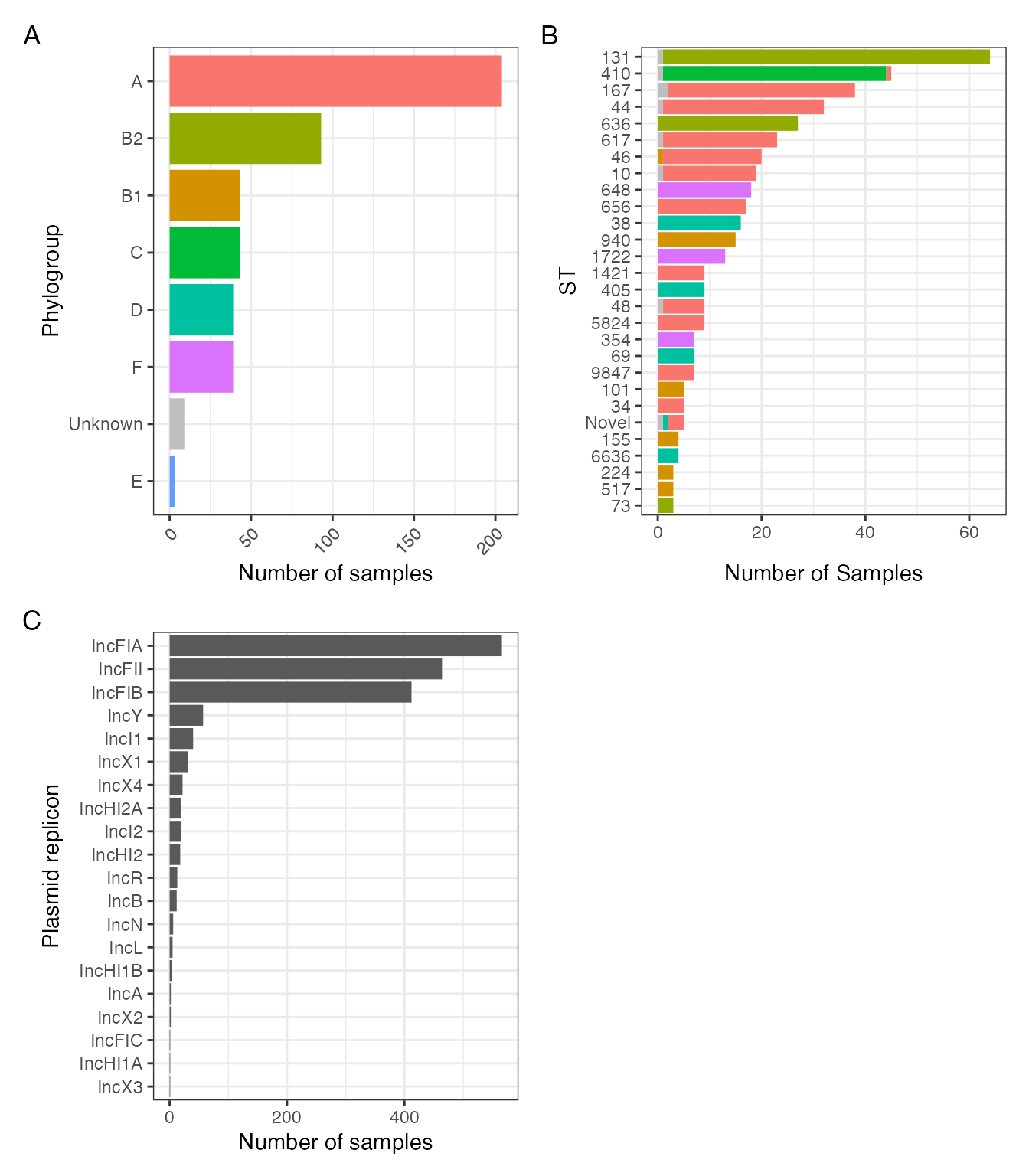
FIGURE 1: Sequence types (A) and phylogroups (B) of included isolates amd (C) identfied Inc-type plasmid replicons.
Compare within- to between- patient diversity
btESBL_sequence_sample_metadata %>%
  filter(species == "E. coli") %>%
  group_by(pid) %>%
  summarise(
    n_sts_per_participant = length(unique(ST)),
    n_samples_per_participant = n()
  ) %>%
  mutate(
    n_samples_per_participant = factor(n_samples_per_participant,
      levels = 1:5
    ),
    n_sts_per_participant = factor(n_sts_per_participant, levels = 1:5)
  ) %>%
  count(n_sts_per_participant, n_samples_per_participant, .drop = FALSE) %>%
  filter(as.numeric(as.character(n_samples_per_participant)) >=
    as.numeric(as.character(n_sts_per_participant))) %>%
  ggplot(aes(n_samples_per_participant, n_sts_per_participant,
    label = n, fill = n, color = -n
  )) +
  geom_tile(color = NA) +
  geom_text() +
  scale_fill_viridis_c() +
  scale_color_gradient(low = "black", high = "white") +
  guides(color = "none") +
  labs(
    x = "No. of samples per participant",
    y = "No. of STs per participant",
    fill = "No. of\nParticipants"
  ) +
  theme_bw() -> samples_vs_st_plot


btESBL_snpdists_esco %>%
  rename(sample1 = sample) %>%
  pivot_longer(-sample1,
    names_to = "sample2",
    values_to = "snpdist"
  ) %>%
  left_join(
    btESBL_sequence_sample_metadata %>%
      filter(species == "E. coli") %>%
      transmute(
        pid1 = pid,
        ST1 = ST,
        sample1 = lane
      )
  ) %>%
  left_join(
    btESBL_sequence_sample_metadata %>%
      filter(species == "E. coli") %>%
      transmute(
        pid2 = pid,
        ST2 = ST,
        sample2 = lane
      )
  ) %>%
  rowwise() %>%
  mutate(filter_var = paste(sort(c(sample1, sample2)), collapse = ",")) -> df
#> Joining with `by = join_by(sample1)`
#> Joining with `by = join_by(sample2)`

df[!duplicated(df$filter_var), ] -> df

df %>%
  filter(sample1 != sample2) %>%
  filter(ST1 == ST2) %>%
  filter(!is.na(pid1) & !is.na(pid2)) %>%
  mutate(btwn_var = if_else(pid1 == pid2, "Within-participant, same ST",
    "Between-participant, same ST"
  )) %>%
  ggplot(aes(snpdist)) +
  # geom_density() +
  geom_histogram(bins = 50, color = "black", size = 0.4) +
  xlim(0, 200) +
  facet_wrap(~btwn_var, scales = "free") +
  theme_bw() +
  guides(fill = "none") +
  labs(
    x = "Core genome SNP distance",
    y = "Number of sample-pairs"
  ) +
  scale_fill_viridis_d(option = "cividis") -> snpdist_plot
#> Warning: Using `size` aesthetic for lines was deprecated in ggplot2 3.4.0.
#> ℹ Please use `linewidth` instead.
#> This warning is displayed once every 8 hours.
#> Call `lifecycle::last_lifecycle_warnings()` to see where this warning was
#> generated.


((samples_vs_st_plot + plot_spacer() + plot_layout(widths = c(1.5,1))) /
  snpdist_plot) +
  plot_annotation(tag_levels = "A") -> within_participant_diversity_plot

within_participant_diversity_plot
#> Warning: Removed 751 rows containing non-finite values (`stat_bin()`).
#> Warning: Removed 4 rows containing missing values (`geom_bar()`).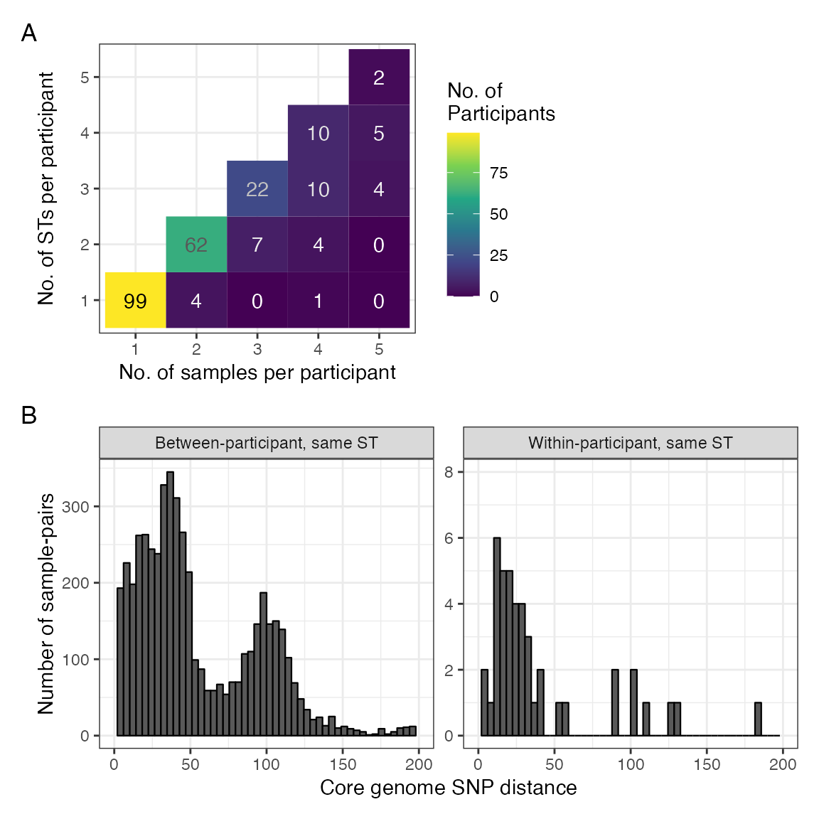
Comparing within- to between- participant diversity. A: Heatmap showing number of samples per participant versus number of STs per participant demonstrating that most participants have either one sample or more than one sample with different STs. B: Histogram of pairwise core genome SNP difference comparing only sample pairs that are of the same ST, stratified by whether sample pair is between-participant (left panel) or within-participant (right panel), demonstrating a similar distribution for each.
Compare phylogroup to horesh collection
As per reviewer’s comments - stratify Horesh collection by invasive vs carriage and ESBL vs not ESBL for comparison
# add esbl status to btESBL_ecoli_horesh_metadata

btESBL_ecoli_horesh_metadata %>%
  left_join(
    btESBL_ecoli_horesh_amr %>%
      left_join(
        select(
          btESBL_NCBI_phenotypic_bl,
          allele_name,
          class
        ),
        by = c("ref_seq" = "allele_name")
      ) %>%
      group_by(ID) %>%
      summarise(res = if_else(
        any(grepl("ESBL|AmpC|Carbapenemase", class)),
        "ESBL/AmpC/Carbapenemase",
        "No ESBL/AmpC/Carbapenemase"
      )),
    by = c("ID" = "ID")
  ) -> btESBL_ecoli_horesh_metadata
bind_rows(
btESBL_ecoli_horesh_metadata %>%
  transmute(Study = "Global",
            Phylogroup = Phylogroup),
btESBL_sequence_sample_metadata %>%
  filter(species == "E. coli") %>%
  transmute(Study = "This Study",
            Phylogroup = ecoli_phylogroup)
) %>%
  mutate(Phylogroup =
           if_else(Phylogroup == "Not Determined",
                   "Unknown",
                   Phylogroup),
         Phylogroup = fct_infreq(Phylogroup)
  ) %>%
  count(Study, Phylogroup, .drop = FALSE) %>%
  group_by(Study) %>%
  mutate(prop = n/sum(n)) %>%
  ggplot(aes(fct_reorder(Phylogroup, prop),
             prop,
             group = Study,
             fill = Study)) +
  geom_col(position = "dodge") +
  theme_bw() +
  theme(axis.text.x = element_text(angle = 45, hjust = 1)) +
  labs(x = "Phylogroup",
       y = "Proportion") ->
  malawi_vs_global_pgroup

malawi_vs_global_pgroup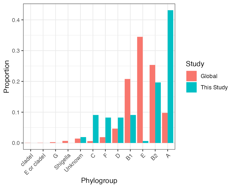
Phylogroup distribution in isolates from this study comapred to the Horesh et al collection
if (write_figs) {
  ggsave(
    here("figures/ecoli-genomics/global_vs_malawi_pgroup.svg"),
    malawi_vs_global_pgroup,
    width = 5,
    height = 4
  )
  ggsave(
    here("figures/ecoli-genomics/global_vs_malawi_pgroup.pdf"),
    malawi_vs_global_pgroup,
    width = 5,
    height = 4
  )
}
bind_rows(
  btESBL_ecoli_horesh_metadata %>%
    transmute(
      Study = "Global",
      Phylogroup = Phylogroup,
      res = res,
      source = case_when(
        Isolation == "Unknown" ~ "Unknown",
        Isolation %in% c("Feces", "Rectal", "Rectal
                                                Swab") ~ "Stool",
        TRUE ~ "Invasive"
      )
    ),
  btESBL_sequence_sample_metadata %>%
    filter(species == "E. coli") %>%
    transmute(
      Study = "This Study",
      Phylogroup = ecoli_phylogroup,
      res = "ESBL/AmpC/Carbapenemase",
      source = "Stool"
    )
) %>%
  mutate(
    Phylogroup =
      case_when(
        Phylogroup == "Not Determined" ~ "Unknown",
        grepl("clade|Shigella", Phylogroup) ~ "Other",
        TRUE ~ Phylogroup
      )
  ) %>%
  filter(!is.na(res)) %>%
  #  mutate(across(everything(), as.factor)) %>% */
  count(Study, Phylogroup, res, source, .drop = FALSE) %>%
  group_by(Study, res, source) %>%
  mutate(prop = n / sum(n),
         source = factor(source,
                      levels = c("Stool","Invasive","Unknown")
         )) %>%
  ggplot(aes(Phylogroup,
    prop,
    group = Study,
    fill = Study
  )) +
  geom_col(position = "dodge") +
  theme_bw() +
  theme(axis.text.x = element_text(angle = 45, hjust = 1)) +
  labs(
    x = "Phylogroup",
    y = "Proportion"
  ) +
  facet_grid(source ~ res) -> malawi_vs_global_pgroup_stratified

malawi_vs_global_pgroup_stratified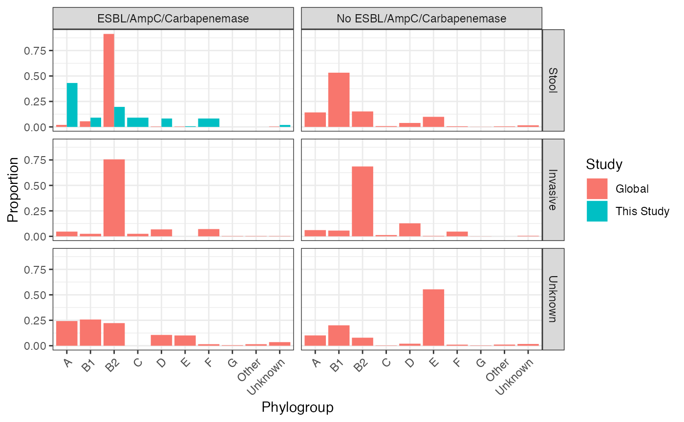
Phylogroup distribution in isolates from this study comapred to the Horesh et al collection, stratified by source of isolation and presence of ESBL/AmpC/carbapenemase gene. Includes only those isolates for which metadata is available to determine source of isolate (n = 3921)
Virulence
- any shiga toxin stx present assign STEC
- if eae is present the assign aEPEC (atypical EPEC)/EPEC;
- if both Shiga-toxin and eae present assign EHEC
- if either aatA, aggR or aaiC present the assign EAEC;
- if est ( sta1 in virulencefinder) or elt (ltcA in virulencefinder) present assign ETEC
- if ipaH9.8 or ipaD, characteristic of the invasive virulence plasmid pINV present assignmen EIEC
Only 2 aEPEC/EPEC, 10 EAEC.
Malawi phylogeny
dassimEcoli_BTEcoli.accession %>%
  as.data.frame() -> dassimEcoli_BTEcoli.accession

rownames(dassimEcoli_BTEcoli.accession ) <-
  dassimEcoli_BTEcoli.accession$lane

 dassimEcoli_BTEcoli.accession %>%
  select(lane, ST) %>%
  group_by(ST) %>%
  mutate(n = n(),
         ST = if_else(n == 1, "Other", ST)) %>%
  mutate(ST = if_else(!ST %in% c("Novel", "Other"),
                      paste0("ST", ST), ST)) %>%
  arrange(fct_infreq(ST)) %>%
  pivot_wider(id_cols = lane,
              names_from = ST,
              values_from = ST,
              values_fn = length,
              values_fill = 0) %>%
  mutate(across(everything(), as.character)
         ) %>%
  relocate(Other, .after = everything()) %>%
  as.data.frame() ->
  mlst_onehot

rownames(mlst_onehot) <- mlst_onehot$lane

(
(
  ggtree(btESBL_coregene_tree_esco) %>%
    gheatmap(
      select(dassimEcoli_BTEcoli.accession, Phylogroup),
      width = 0.05,
      color = NA,
      font.size = 3,
      colnames_angle = 90,
      colnames_position = "top",
      colnames_offset_y = 3,
      hjust = 0
    ) +
    scale_fill_manual(
      values = hue_pal()(8),
      name = "Phylogroup") +
   new_scale_fill()
) %>%
  gheatmap(select(mlst_onehot, -lane),
           font.size = 2.5,
           color = NA,
           colnames_angle = 90,
           offset = .0022,
           colnames_offset_y = 3,
           colnames_position = "top",
           hjust = 0)  +
    scale_fill_manual(values = c("lightgrey", "black"), guide = "none") +
    new_scale_fill()
  ) %>%
  gheatmap(select(dassimEcoli_BTEcoli.accession, Pathotype),
           width = 0.05,
           font.size = 3,
           color = NA,
           colnames_angle = 90,
           offset = .001,
           colnames_offset_y = 3,
           colnames_position = "top",
           hjust = 0)  +
  scale_fill_manual(values = viridis_pal(option = "plasma")(6)[c(3,5)],
                    name = "Pathotype",
                    na.translate = FALSE) +
  ylim(NA, 540) +
  annotate("text", x = 0.03, y = 520, label = "Sequence Type",
           size = 3) -> malawi_treeplot
#> Scale for fill is already present.
#> Adding another scale for fill, which will replace the existing scale.
#> Scale for fill is already present.
#> Adding another scale for fill, which will replace the existing scale.
#> Scale for fill is already present.
#> Adding another scale for fill, which will replace the existing scale.
#> Scale for y is already present.
#> Adding another scale for y, which will replace the existing scale.


malawi_treeplot
SUPPLEMENTARY FIGURE 1: Midpoint-rooted maximum-likelohood phylogeny of study isolates showing phylogroup and multilocus sequence type.
AMR determinants
# add class ro which resistnce is conferred --------------------------------

quinolone <- "Par|Gyr|Par|Qnr|Qep|Nor|GyrA|GyrB|ParC|ParE"
tetracycline <- "Tet"
sulphonamide <- "Sul"
aminoglycoside <- "Str|Aad|Aac|Aph|Rmt|APH"
streptothricin <- "Sat"
macrolide <- "Mph|Mdf|Erm|Ere"
fosfomycin <- "Fos"
chloramphenicol <- "Cat|FloR|Cml"
trimethoprim <- "Dfr"
rifampicin <- "Arr"
ESBL <- "SHV_12"
penicillinase <- "OKP|SCO|LEN|LAP"
ampc <- "CMY"

btESBL_amrgenes %>%
  semi_join(dassimEcoli_BTEcoli.accession,
            by = c( "lane")) %>%
  select(-genus) %>%
  rename(gene = ref_seq) %>%
  # add in QRDR mutations
  bind_rows(
    btESBL_qrdr_mutations %>%
      filter(genus == "E. coli") %>%
      select(-genus) %>%
      semi_join(
        btESBL_CARD_qrdr_mutations,
        by = c("variant" = "variant",
              "gene" =  "gene")
      ) %>%
      select(gene, lane) %>%
      unique() %>%
      mutate(gene =
               gsub("(^.{1})", '\\U\\1',
                    gene,
                    perl = TRUE))
      ) %>%
  filter(!grepl("AmpH|AMPH|AmpC|MrdA|MefB", gene)) %>%
  # add in beta-lactamases
  left_join(
    select(btESBL_NCBI_phenotypic_bl, allele_name, class),
    by = c("gene" = "allele_name")) %>%
  mutate(class = case_when(
    str_detect(gene, quinolone) ~ "Quinolone",
    str_detect(gene, tetracycline) ~ "Tetracycline",
    str_detect(gene, sulphonamide) ~ "Sulphonamide",
    str_detect(gene, aminoglycoside) ~ "Aminoglycoside",
    str_detect(gene, streptothricin) ~ "Streptothricin",
    str_detect(gene, macrolide) ~ "Macrolide",
    str_detect(gene, fosfomycin) ~ "Fosfomycin",
    str_detect(gene, chloramphenicol) ~ "Chloramphenicol",
    str_detect(gene, rifampicin) ~ "Rifampicin",
    str_detect(gene,trimethoprim) ~ "Trimethoprim",
    str_detect(gene,ESBL) ~ "ESBL",
    str_detect(gene,penicillinase) ~ "Penicillinase",
    str_detect(gene,ampc) ~ "AmpC",
    TRUE ~ class
  )) %>%
  mutate(gene = if_else(gene == "TEM_95",
                        "TEM_1",
                        gene)) ->
  amr

### plot prevalence ----------------------------------------


amr %>%
  group_by(class) %>%
  mutate(n_class = length(class),
         n_genes_in_class = n_distinct(gene)) %>%
  select(class, n_class,n_genes_in_class) %>%
  unique() %>%
  arrange(n_class) %>%
  ungroup() %>%
  mutate(end = cumsum(n_genes_in_class),
         start = lag(end, default = 0),
         textpos = start + 0.6 + 0.5 * (end - start)) -> annotate.df

amr %>%
  group_by(class) %>%
  mutate(n_class = length(class),
         n_genes_in_class = n_distinct(gene),
         gene = gsub("_", "-", gene)) %>%
ggplot( aes(fct_reorder(fct_rev(fct_infreq(gene)), n_class),
            fill = class)) +
  geom_bar() +
  theme_bw() +
  coord_flip(ylim = c(-5,450),clip = "off", expand = FALSE, xlim = c(0, 76)) +
  annotate(geom = "segment",
             x = annotate.df$start + 0.5 + 0.2,
             xend = annotate.df$end + 0.5 - 0.2,
             y = -115, yend = -115 ) +
  annotate(geom = "text", y = -125,
           x = annotate.df$textpos,
           label = annotate.df$class,
           size = 3,
           hjust = 1) +
  labs(y = "Number of samples") +
  theme(plot.margin = unit(c(0.2,0.5,0.2,4), "cm"),
        axis.title.y  = element_blank(),
        legend.position = "none") -> amrplot

amrplot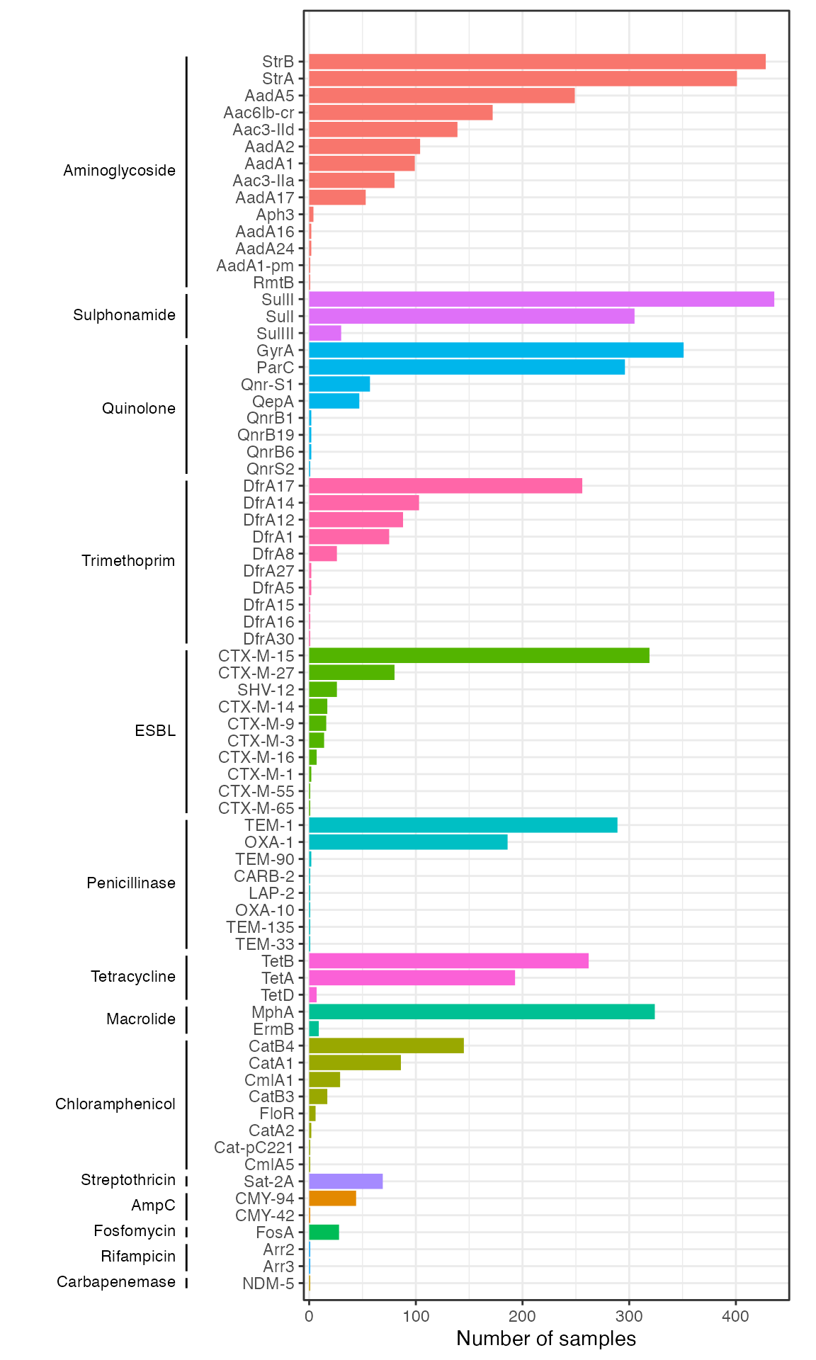
if (write_figs) {
  ggsave(
    filename = here("figures/ecoli-genomics/amr_plot.pdf"),
    plot = amrplot,
    width = 6,
    height = 10
  )
  ggsave(
    filename = here("figures/ecoli-genomics/amr_plot.svg"),
    plot = amrplot,
    width = 6,
    height = 10
  )
}
AMR mapped to tree
amr %>%
  # filter(!gene %in% c("OqxA", "OqxB", "FosA")) %>%
  # remove FosA as not in KpI which we are plottingh
  mutate(
         gene = gsub("_","-", gene)) %>%
  group_by(class) %>%
  mutate(n_class = length(class)) %>%
  ungroup() %>%
  group_by(gene) %>%
  mutate(n_gene = length(gene)) %>%
  arrange(desc(n_class), desc(n_gene)) %>%
  select(-n_class, -n_gene) %>%
  pivot_wider(id_cols = lane,
              values_from = class,
              names_from = gene) %>%

  as.data.frame() ->
  amr.ariba.maptotree


amr %>%
    # filter(!gene %in% c("OqxA", "OqxB", "FosA")) %>%
    mutate(
           gene = gsub("_","-", gene)) %>%
    group_by(class) %>%
    mutate(n_class = length(class)) %>%
    ungroup() %>%
    group_by(gene) %>%
    mutate(n_gene = length(gene)) %>%
    arrange(desc(n_class), desc(n_gene)) %>% pull(class) %>%
  unique() -> class_order

rownames(amr.ariba.maptotree) <- amr.ariba.maptotree$lane

colz = hue_pal()(13)
names(colz) <- sort(unique(amr %>%
                             filter(class != "Fosfomycin") %>%
                             pull(class)))

ggtree(btESBL_coregene_tree_esco ) %>%
#ggtree(tree) %>%
    gheatmap(
        select(amr.ariba.maptotree,-lane),
        width = 5,
        color = NA,
        font.size = 3,
        colnames_angle = 90,
        colnames_position = "top",
        colnames_offset_y = 0,
        hjust = 0,
        offset = 0
    ) +
  ylim(NA, 500) +
  scale_fill_manual(name = "Class", values = colz,
                    breaks = class_order,
                    na.translate = FALSE) ->
  malawi_tree_with_amr
#> Scale for y is already present.
#> Adding another scale for y, which will replace the existing scale.
#> Scale for fill is already present.
#> Adding another scale for fill, which will replace the existing scale.

malawi_tree_with_amr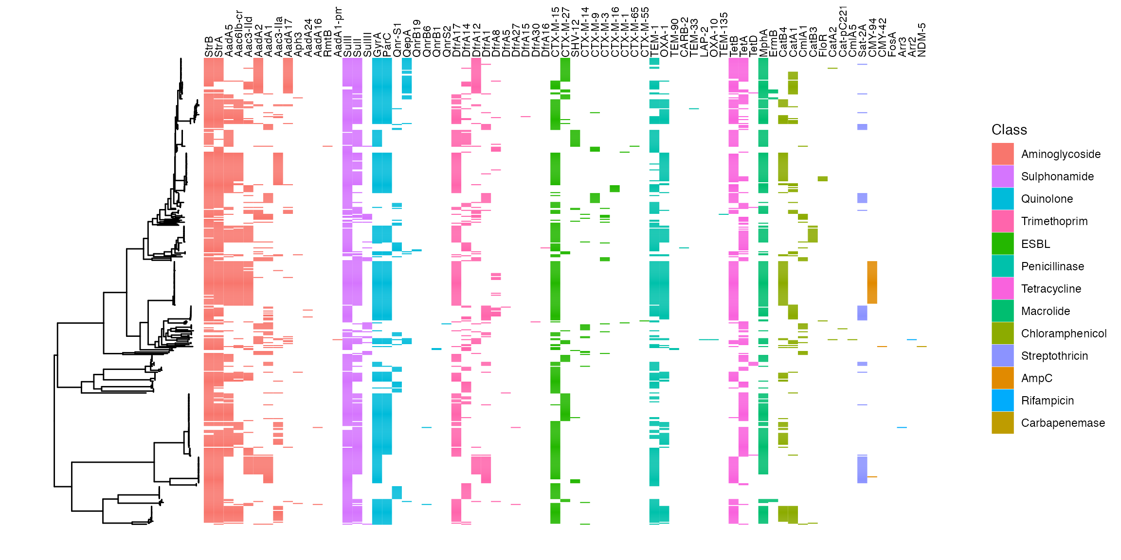
AMR determinants mapped back to phylogeny
Malawi isolates in a global context
Phylogeny
 #prepare metadata ----------
# lookup list of horesh merged clusters


purrr::map_df(
  unique(grep("_", btESBL_ecoli_global_popPUNK_clusters$Cluster, value = TRUE)),
              function(x)
                data.frame(mergeclust = x,
                           splts = strsplit(x, "_")[[1]])) %>%
  mutate(splts = as.numeric(splts)) -> mergclust_lookup

bind_rows(
  dassimEcoli_BTEcoli.accession %>%
    transmute(
      lane = lane,
      ST = ST,
      Phylogroup = Phylogroup,
      study = "dassim",
      Country = "Malawi",
      Continent = "Africa",
      Year = year(data_date),
      res = "ESBL/AmpC/Carbapenemase",
      source = "Colonising"
    ) %>%
    left_join(
      btESBL_ecoli_global_popPUNK_clusters,
      by = "lane"
    ),
  btESBL_ecoli_musicha_metadata %>%
    transmute(
      lane = lane,
      Cluster = Cluster,
      ST = if_else(is.na(ST),
        "Novel",
        as.character(ST)
      ),
      Phylogroup = phylogroup,
      study = "musicha",
      Country = "Malawi",
      Continent = "Africa",
      Year = Year
    ),
  btESBL_ecoli_horesh_metadata %>%
    mutate(
      assembly_name_recode =
        gsub("\\..*$", "", Assembly_name)
    ) %>%
    left_join(mergclust_lookup, by = c("PopPUNK" = "splts")) %>%
    transmute(
      lane = gsub(
        "#",
        "_",
        if_else(
          !is.na(name_in_presence_absence),
          name_in_presence_absence,
          assembly_name_recode
        )
      ),
      Cluster = if_else(!is.na(mergeclust),
        mergeclust,
        as.character(PopPUNK)
      ),
      ST = gsub("~", "", ST),
      Phylogroup = Phylogroup,
      study = "horesh",
      Country = Country,
      Continent = Continent,
      Year = case_when(
        Year == "Unknown" ~ NA_real_,
        grepl("s", Year) ~ as.numeric(gsub("s", "", Year)),
        grepl("-", Year) ~ as.numeric(gsub("-.*$", "", Year)),
        TRUE ~ as.numeric(str_trim(Year))
      ),
      Pathotype = Pathotype,
      res = res,
      source = case_when(
        Isolation == "Unknown" ~ "Unknown",
        Isolation %in% c("Feces", "Rectal", "Rectal
                                                Swab") ~ "Colonising",
        TRUE ~ "Infecting"
      )
    )
) %>%
  mutate(
    Continent =
      case_when(
        grepl("America", Continent) ~ "Americas",
        is.na(Continent) ~ "Unknown",
        TRUE ~ Continent
      )
  ) %>%
  mutate(
    cluster_recode =
      if_else(
        !grepl(
          paste(c(
            "\\<1", 2:1153, "1184\\>"
          ), collapse = "\\>|\\<"),
          Cluster
        ) &
          !grepl("_", Cluster),
        NA_character_,
        Cluster
      ),
    cluster_recode = factor(
      cluster_recode,
      levels =
        unique(cluster_recode)[
          order(
            as.numeric(
              gsub("_.*$", "", unique(cluster_recode))
            )
          )
        ]
    ),
    Phylogroup =
      case_when(
        Phylogroup %in% c(
          "Unknown", "Not Determined",
          "E or cladeI"
        ) ~
        "Unknown",
        is.na(Phylogroup) ~ "Unknown",
        TRUE ~ Phylogroup
      )
  ) -> df_all
#> Warning: There were 3 warnings in `transmute()`.
#> The first warning was:
#> ℹ In argument: `Year = case_when(...)`.
#> Caused by warning:
#> ! NAs introduced by coercion
#> ℹ Run `dplyr::last_dplyr_warnings()` to see the 2 remaining warnings.
df_all <- as.data.frame(df_all)

write_csv(df_all, here("tables/ecoli-genomics/horesh_globaltree_metadata.csv"))

rownames(df_all) <- df_all$lane
#define color palettes

pgroup_cols <- c(brewer_pal(type = "qual", palette = 8)(10),
                            "white")
  names(pgroup_cols) <- sort(unique(df_all$Phylogroup))

continent_cols <- c(viridis_pal(option = "plasma")(5),
                    "white")
names(continent_cols) <- sort(unique(df_all$Continent))

country_cols <-
  c("Malawi" =  "grey15",
    "Not Malawi" = "lightgrey")

btESBL_ecoli_globaltree -> horesh_context_tree

popPUNK_clusts_inplots <-
  df_all %>%
   filter(lane %in%
           c(tree_subset(
             btESBL_ecoli_globaltree,
             3555, levels_back = 0)$tip.label,
             tree_subset(
               btESBL_ecoli_globaltree,
               5404, levels_back = 0)$tip.label,
             tree_subset(
               btESBL_ecoli_globaltree,
               5652, levels_back = 0)$tip.label)
  ) %>%
  select(cluster_recode) %>%
  unique() %>%
  arrange(cluster_recode) %>%
  pull(cluster_recode)


popPUNK_cols <- c(
  "dodgerblue2", "#E31A1C", # red
  "green4",
  "#6A3D9A", # purple
  "#FF7F00", # orange
  "black", "gold1",
  "skyblue2", "#FB9A99", # lt pink
  "palegreen2",
  "#CAB2D6", # lt purple
  "#FDBF6F", # lt orange
  "gray70", "khaki2",
  "maroon", "orchid1", "deeppink1", "blue1", "steelblue4",
  "darkturquoise", "green1", "yellow4", "yellow3",
  "darkorange4", "brown"
)


#   c(
#   "palegreen2",
#   "#E31A1C",
#   "green4",
#   "#6A3D9A",
#   "#FF7F00",
#   "steelblue4",
#   "gold1",
#   "skyblue2",
#   "dodgerblue2",
#   "#FDBF6F",
#   "gray70",
#   "maroon",
#   "orchid1",
#   "darkturquoise",
#   "darkorange4",
#   "brown",
#   "white"
# )


names(popPUNK_cols) <- df_all %>%
  filter(lane %in%
           c(tree_subset(
             btESBL_ecoli_globaltree,
             3565, levels_back = 0)$tip.label,
             tree_subset(
               btESBL_ecoli_globaltree,
               5404, levels_back = 0)$tip.label,
             tree_subset(
               btESBL_ecoli_globaltree,
               5652, levels_back = 0)$tip.label)
  ) %>%
  select(cluster_recode) %>%
  unique() %>%
  arrange(cluster_recode) %>%
  pull(cluster_recode)

popPUNK_cols <- popPUNK_cols[!is.na(names(popPUNK_cols))]


offset_add <- 0

(
    (
      (
        (
          ggtree(btESBL_ecoli_globaltree, size = 0.2) %<+%
            (select(df_all, lane, ST) %>%
               mutate(
                 ST = if_else(ST == 167,
                              as.character("hilight"), NA_character_)
               ))  %>%
            gheatmap(
              select(df_all, `Year`),
              font.size = 4,
              width = 0.03,
              colnames_position = "top",
              color = NA,
              colnames_offset_y = 5,
              colnames_angle = 90,
              offset = 0.0006 + offset_add,
              hjust = 0
            )  +
            scale_fill_viridis_c(name = "Year", na.value = "white",
                                 guide = guide_colorbar(order = 2)) +
            new_scale_fill()
        ) %>%
          gheatmap(
            select(df_all, Continent),
            font.size = 4,
            width = 0.03,
            colnames_position = "top",
            color = NA,
            colnames_offset_y = 5,
            colnames_angle = 90,
            offset = 0.0012 + offset_add,
            hjust = 0
          ) +
          scale_fill_manual(values =
                              continent_cols,
                            name = "Continent",
                            guide = guide_legend(order = 3)) +
          new_scale_fill()
      ) %>%
        gheatmap(
          select(df_all, Country) %>%
            mutate(Country = if_else(
              Country == "Malawi",
              "Malawi", "Not Malawi"
            )),
          font.size = 4,
          width = 0.03,
          colnames_position = "top",
          color = NA,
          colnames_offset_y = 5,
          colnames_angle = 90,
          offset = 0.0018 + offset_add,
          hjust = 0
        ) +
        scale_fill_manual(values = country_cols,
                          name = "Country",
                          guide = guide_legend(order = 4)) +
        new_scale_fill()
    ) %>%
      gheatmap(
        select(df_all, Phylogroup) %>%
          mutate(Phylogroup = if_else(
            is.na(Phylogroup) ,"Unknown",
            Phylogroup)),
        width = 0.03,
        color = NA,
        font.size = 4,
        colnames_angle = 90,
        colnames_position = "top",
        colnames_offset_y = 3,
        hjust = 0,
        offset = 0 + offset_add
      ) +
      scale_fill_manual(values = pgroup_cols,
      name = "Phylogroup",
      na.translate = FALSE,
      guide = guide_legend(order = 1)) +
      new_scale_fill()
  ) +
    ylim(NA, 3550) +# + geom_tippoint(aes(color = ST)) +
    geom_treescale(y = 2366, x = 0.004,offset = 30)  -> p
#> Scale for fill is already present.
#> Adding another scale for fill, which will replace the existing scale.
#> Scale for fill is already present.
#> Adding another scale for fill, which will replace the existing scale.
#> Scale for fill is already present.
#> Adding another scale for fill, which will replace the existing scale.
#> Scale for fill is already present.
#> Adding another scale for fill, which will replace the existing scale.
#> Scale for y is already present.
#> Adding another scale for y, which will replace the existing scale.

  p + geom_hilight( node = 3565, alpha = 0.3,
                    fill = "steelblue",
                    color = NA) +  # phylogroup A
    geom_cladelabel(node = 3565, label = "C", barsize = 0,offset = 0) +
    geom_highlight(node = 5404, alpha = 0.3, fill = "steelblue",
                   color = NA, extend = 0.0002) + # st 410 and context
    geom_cladelabel(node = 5404, label = "B", barsize = 0,offset = 0) +
    geom_highlight(node = 5652, alpha = 0.3, fill = "steelblue",
                   color = NA) + # ST131
    geom_cladelabel(node = 5652, label = "D", barsize = 0,offset = 0) -> p

  # phylo a subreee -----------


offset_add <- 0.0000 #0.0015
textsize <-  3
cladelab_offset <- 0.0001
tippoint_alpha = 0.7

(
  ggtree(
    tree_subset(
      btESBL_ecoli_globaltree, 3565, levels_back = 0)
    ) %<+% select(df_all, lane, cluster_recode) %>%
    gheatmap(
    select(df_all, Country) %>%
      mutate(Country = if_else(
        Country == "Malawi",
        "Malawi", "Not Malawi")),
    font.size = 3,
    width = 0.04,
    colnames_position = "top",
    color = NA,
    colnames_offset_y = 0,
    colnames_angle = 90,
    offset = offset_add,
    hjust = 0
    ) +
    scale_fill_manual(
      values = country_cols,
      name = "Country",
      guide = "none") +
      guides(fill = "none") +
      new_scale_fill()
) +
   ylim(NA, 100) +
   geom_tippoint(aes(color = cluster_recode),
                na.rm = TRUE,
                size = 1,
                alpha = tippoint_alpha) +
  scale_color_manual(name = "PopPUNK\nCluster",
                       values = popPUNK_cols,
                       na.translate = FALSE) +
  geom_treescale(y = 66,
                 x = 0.00005,
                 offset  = 2,
                 width = 0.00001) -> p_phylo_a_subtree
#> Scale for fill is already present.
#> Adding another scale for fill, which will replace the existing scale.
#> Scale for y is already present.
#> Adding another scale for y, which will replace the existing scale.

p_phylo_a_subtree +
  geom_cladelabel(node = 119, label = "ST167",
                  fontsize = textsize,
                  offset = 0.00002,
                  offset.text = 0.000005) +
  geom_cladelabel(node = 99, label = "ST167",
                  fontsize = textsize,
                  offset = 0.0001665,
                  offset.text = 0.000005) +
  theme(legend.position = "bottom")  +
  guides(
    color = guide_legend(
      nrow = 2,
      byrow = TRUE,
      override.aes = list(alpha = 1))
    ) ->
  plot_phyloa_subtree

# ST131 zoom

offset_add <- 0.0004
(
  ggtree(
    tree_subset(
      btESBL_ecoli_globaltree, 5652, levels_back = 0)
    ) %<+% select(df_all, lane, cluster_recode) %>%
    gheatmap(
      select(df_all, Country) %>%
      mutate(Country = if_else(
        Country == "Malawi",
        "Malawi", "Not Malawi")),
      font.size = 3,
      width = 0.07,
      colnames_position = "top",
      color = NA,
      colnames_offset_y = 0,
      colnames_angle = 90,
      offset =  offset_add,
      hjust = 0
    ) +
    scale_fill_manual(values = country_cols,
                        name = "Country",
                        guide = "none") +
    new_scale_fill()
) +
  ylim(NA, 125) +
  geom_tippoint(aes(color = cluster_recode),
                na.rm = TRUE,
                size = 1,
                alpha = tippoint_alpha) +
  scale_color_manual(name = "PopPUNK\nCluster",
                     values = popPUNK_cols,
                     na.translate = FALSE) +
  geom_treescale(y = 83,
                 x = 0.0001,
                 offset  = 3.6,
                 width = 0.0001) -> p_st131_subtree
#> Scale for fill is already present.
#> Adding another scale for fill, which will replace the existing scale.
#> Scale for y is already present.
#> Adding another scale for y, which will replace the existing scale.

p_st131_subtree +
  geom_cladelabel(node = 104, label = "ST131",
                  fontsize = textsize,
                  offset = 0.0001,
                  offset.text = 0.00002) +
  theme(legend.position = "bottom") +
  guides(color = guide_legend(
    nrow = 2,
    byrow = TRUE,
    override.aes = list(alpha = 1))
    ) -> plot_st131tree

# st410 subtree


offset_add <- 0.00007
# offset_multiple <- 0.00008

(
  ggtree(
    tree_subset(
      btESBL_ecoli_globaltree, 5404, levels_back = 0)
    ) %<+% select(df_all, lane, cluster_recode) %>%
    gheatmap(
    select(df_all, Country) %>%
      mutate(Country = if_else(
        Country == "Malawi",
        "Malawi", "Not Malawi")),
    font.size = 3,
    width = 0.055,
    colnames_position = "top",
    color = NA,
    colnames_offset_y = 0,
    colnames_angle = 90,
    offset = offset_add,
    hjust = 0,
    ) +
    scale_fill_manual(values = country_cols,
                      name = "Country",
                      guide = "none") +
    new_scale_fill()
) +
  ylim(NA, 60) +
  geom_tippoint(aes(color = cluster_recode),
                na.rm = TRUE,
                size = 1,
                alpha = tippoint_alpha) +
  scale_color_manual(name = "PopPUNK\nCluster",
                     values = popPUNK_cols,
                     na.translate = FALSE) +
  geom_treescale(y = 40,
                 x = offset_add/2,
                 offset  = 1,
                 width = 0.00001) -> p_st410_subtree
#> Scale for fill is already present.
#> Adding another scale for fill, which will replace the existing scale.
#> Scale for y is already present.
#> Adding another scale for y, which will replace the existing scale.

p_st410_subtree +
  geom_cladelabel(48, label = "ST410",
                  fontsize = textsize,
                  offset = offset_add/5,
                  offset.text = 0.000002) +
  theme(legend.position = "bottom")  +
  guides(
    color = guide_legend(
      nrow = 2, byrow = TRUE,
         override.aes = list(alpha = 1)
      )
    ) -> plot_st410tree

(plot_st410tree + plot_phyloa_subtree + plot_st131tree) +
  plot_annotation(tag_levels = "A") + plot_layout(guides = "collect") &
  theme(legend.position = "bottom")   -> subtreesplot

p / (subtreesplot) + plot_annotation(tag_levels = "A") +
  plot_layout(guides = "collect", heights = c(2.5,1)) -> global_tree_plot

# height 12, width 9 loooks gooooooood
global_tree_plot
#> Warning: The following aesthetics were dropped during statistical transformation: node,
#> parent
#> ℹ This can happen when ggplot fails to infer the correct grouping structure in
#>   the data.
#> ℹ Did you forget to specify a `group` aesthetic or to convert a numerical
#>   variable into a factor?
#> The following aesthetics were dropped during statistical transformation: node,
#> parent
#> ℹ This can happen when ggplot fails to infer the correct grouping structure in
#>   the data.
#> ℹ Did you forget to specify a `group` aesthetic or to convert a numerical
#>   variable into a factor?
#> The following aesthetics were dropped during statistical transformation: node,
#> parent
#> ℹ This can happen when ggplot fails to infer the correct grouping structure in
#>   the data.
#> ℹ Did you forget to specify a `group` aesthetic or to convert a numerical
#>   variable into a factor?
#> The following aesthetics were dropped during statistical transformation: node,
#> parent
#> ℹ This can happen when ggplot fails to infer the correct grouping structure in
#>   the data.
#> ℹ Did you forget to specify a `group` aesthetic or to convert a numerical
#>   variable into a factor?
#> The following aesthetics were dropped during statistical transformation: node,
#> parent
#> ℹ This can happen when ggplot fails to infer the correct grouping structure in
#>   the data.
#> ℹ Did you forget to specify a `group` aesthetic or to convert a numerical
#>   variable into a factor?
#> The following aesthetics were dropped during statistical transformation: node,
#> parent
#> ℹ This can happen when ggplot fails to infer the correct grouping structure in
#>   the data.
#> ℹ Did you forget to specify a `group` aesthetic or to convert a numerical
#>   variable into a factor?
#> The following aesthetics were dropped during statistical transformation: node,
#> parent
#> ℹ This can happen when ggplot fails to infer the correct grouping structure in
#>   the data.
#> ℹ Did you forget to specify a `group` aesthetic or to convert a numerical
#>   variable into a factor?
#> The following aesthetics were dropped during statistical transformation: node,
#> parent
#> ℹ This can happen when ggplot fails to infer the correct grouping structure in
#>   the data.
#> ℹ Did you forget to specify a `group` aesthetic or to convert a numerical
#>   variable into a factor?
#> The following aesthetics were dropped during statistical transformation: node,
#> parent
#> ℹ This can happen when ggplot fails to infer the correct grouping structure in
#>   the data.
#> ℹ Did you forget to specify a `group` aesthetic or to convert a numerical
#>   variable into a factor?
#> The following aesthetics were dropped during statistical transformation: node,
#> parent
#> ℹ This can happen when ggplot fails to infer the correct grouping structure in
#>   the data.
#> ℹ Did you forget to specify a `group` aesthetic or to convert a numerical
#>   variable into a factor?
#> The following aesthetics were dropped during statistical transformation: node,
#> parent
#> ℹ This can happen when ggplot fails to infer the correct grouping structure in
#>   the data.
#> ℹ Did you forget to specify a `group` aesthetic or to convert a numerical
#>   variable into a factor?
#> The following aesthetics were dropped during statistical transformation: node,
#> parent
#> ℹ This can happen when ggplot fails to infer the correct grouping structure in
#>   the data.
#> ℹ Did you forget to specify a `group` aesthetic or to convert a numerical
#>   variable into a factor?
#> The following aesthetics were dropped during statistical transformation: node,
#> parent
#> ℹ This can happen when ggplot fails to infer the correct grouping structure in
#>   the data.
#> ℹ Did you forget to specify a `group` aesthetic or to convert a numerical
#>   variable into a factor?
#> The following aesthetics were dropped during statistical transformation: node,
#> parent
#> ℹ This can happen when ggplot fails to infer the correct grouping structure in
#>   the data.
#> ℹ Did you forget to specify a `group` aesthetic or to convert a numerical
#>   variable into a factor?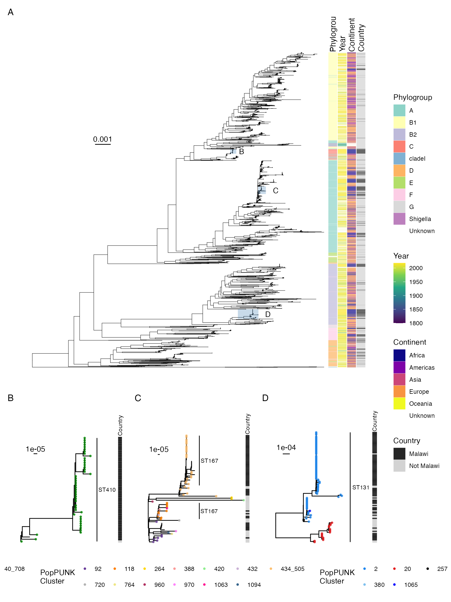
A: Malawian E. coli isolates in a global phylogeny. All genomes from Musicha et al along with 500 context genomes from Horesh et al are included. Heatmaps show Phylogroup, year of collection, continent of collection and country (Malawi vs other). Highlighted areas and subtrees B-D show the phylogenetic context of the three commonest STs in this study: ST410 (B), ST167 (C) and ST131 (D). The tree tips in the subtree plots are coloured by popPUNK cluster assignment, with novel clusters that were not identified in the original Horesh collection given no color.
PopPUNK clusters
df_all %>%
  filter(study %in% c("dassim", "horesh")) %>%
  mutate(res = if_else(grepl("No", res), "No ESBL", "ESBL")) %>%
  group_by(study) %>%
  mutate(n_tot_study = n()) %>%
  group_by(Cluster, study) %>%
  summarise(
    n_cluster = n(),
    prop_cluster = n_cluster / unique(n_tot_study)
  ) %>%
  group_by(Cluster) %>%
  mutate(n_studies_cluster_is_in = length(Cluster)) %>%
  filter(
    grepl(
      paste(c("\\<1", 2:49, "50\\>"), collapse = "\\>|\\<"),
      Cluster
    ) |
      n_studies_cluster_is_in > 1 |
      study == "dassim"
  ) %>%
  filter(!(study == "dassim" & n_cluster <= 3 & n_studies_cluster_is_in == 1)) %>%
  ungroup() %>%
  mutate(
    prop_cluster =
      if_else(
        study == "dassim",
        -1 * prop_cluster,
        prop_cluster
      ),
    Cluster = factor(
      Cluster,
      levels =
        unique(Cluster)[
          order(
            as.numeric(
              gsub("_.*$", "", unique(Cluster))
            )
          )
        ]
    )
  ) %>%
  mutate(
    study = case_when(
      study == "dassim" ~ "This Study",
      TRUE ~ "Horesh et al."
    ),
    study = factor(study, levels = c("This Study", "Horesh et al."))
  ) %>%
  ggplot(aes(x = prop_cluster, y = fct_rev(Cluster), fill = study)) +
  geom_col(color = "black", size = 0.2) +
  theme_bw() +
  labs(
    y = "PopPUNK cluster", fill = "",
    x = "Proportion of samples"
  ) +
  scale_x_continuous(labels = c(0.1, 0.0, 0.1, 0.2, 0.3)) +
  scale_fill_manual(values = c(
    viridis_pal(option = "cividis")(8)[c(2)],
    "grey60"
  )) +
  theme(
    axis.text.y = element_text(size = 5),
    axis.text.x = element_text(size = 7),
    legend.position = "bottom"
  ) -> p1
#> `summarise()` has grouped output by 'Cluster'. You can override using the
#> `.groups` argument.

df_all %>%
  filter(study %in% c("dassim", "horesh")) %>%
  mutate(
    study = case_when(
      study == "dassim" ~ "This Study",
      TRUE ~ "Horesh Collection"
    ),
    study = factor(study, levels = c("This Study", "Horesh Collection"))
  ) %>%
  mutate(Cluster = factor(
    Cluster,
    levels =
      unique(Cluster)[
        order(
          as.numeric(
            gsub("_.*$", "", unique(Cluster))
          )
        )
      ]
  )) %>%
  ggplot(aes(Cluster, color = study, group = study)) +
  stat_ecdf(pad = TRUE, geom = "step") +
  scale_x_discrete(
    breaks = as.character(c(1, seq(from = 100, to = 1400, by = 100))),
    expand = c(0.01, 0.01)
  ) +
  theme_bw() +
  labs(
    y = "Cumulative proportion",
    x = "PopPUNK cluster", color = ""
  ) +
  geom_vline(
    xintercept = "1184",
    alpha = 0.8,
    linetype = "dotted"
  ) +
  scale_color_manual(
    values = c(
      viridis_pal(option = "cividis")(8)[c(2)],
      "grey60"
    ),
    guide = "none"
  ) +
  theme(
    axis.text.y = element_text(size = 7),
    axis.text.x = element_text(angle = 45, hjust = 1, size = 5),
    legend.position = "none"
  ) -> p2

  (
    p1 +
      (p2 + plot_spacer() + plot_layout(ncol = 1))
  ) + plot_layout(ncol = 2, guides = "collect") +
    plot_annotation(tag_levels = "A") &
    theme(legend.position = "bottom") -> pp_cluster_plots

  pp_cluster_plots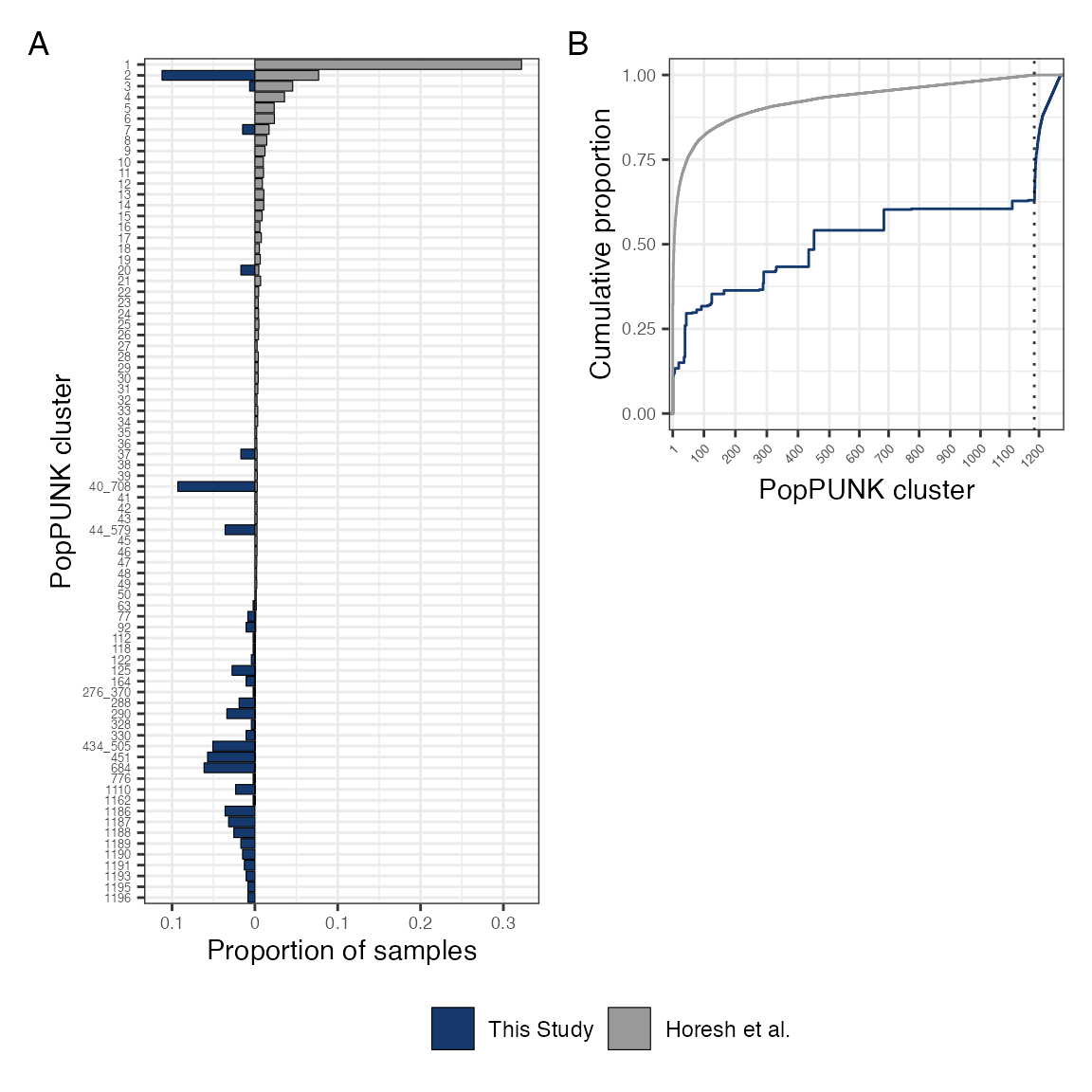
PopPUNK cluster assignments of isolates from this study, using the Horesh et al database. A: Proportion of samples assigned to a given cluster for this study (left) and the Horesh collection (right); clusters are ordered numerically which by definition is form largest to smallest in the Horesh collection. B: Cumulative proportion of isolates with cluster membership, with clusters again ordered numerically (i.e. largest to smallest). Dotted line indicates the end of clusters defined in the original Horesh popPUNK database; clusters to the right of this line are newly defined in the isolates in this study.
if (write_figs) {
  ggsave(
    here("figures/ecoli-genomics/global_poppunk_clusterplot.pdf"),
    pp_cluster_plots,
    width = 6,
    height = 6
  )
  ggsave(
    here("figures/ecoli-genomics/global_poppunk_clusterplot.svg"),
    pp_cluster_plots,
    width = 6,
    height = 6
  )
}
# get clusters to include


df_all %>%
  mutate(res = if_else(grepl("No", res), "No ESBL", "ESBL")) %>%
  filter(study %in% c("dassim", "horesh")) %>%
  group_by(study) %>%
  mutate(n_tot_study = n()) %>%
  group_by(Cluster, study) %>%
  summarise(
    n_cluster = n(),
    prop_cluster = n_cluster / unique(n_tot_study)
  ) %>%
  group_by(Cluster) %>%
  mutate(n_studies_cluster_is_in = length(Cluster)) %>%
  filter(
    grepl(
      paste(c("\\<1", 2:49, "50\\>"), collapse = "\\>|\\<"),
      Cluster
    ) |
      n_studies_cluster_is_in > 1 |
      study == "dassim"
  ) %>%
  filter(!(study == "dassim" &
           n_cluster <= 3 & n_studies_cluster_is_in == 1)) %>%
  ungroup() %>%
  pull(Cluster) %>%
  unique() -> clusters_to_include
#> `summarise()` has grouped output by 'Cluster'. You can override using the
#> `.groups` argument.

df_all %>%
  mutate(res = if_else(grepl("No", res), "No ESBL", "ESBL")) %>%
  filter(study %in% c("dassim", "horesh")) %>%
  group_by(study) %>%
  filter(source != "Unknown") %>%
  mutate(n_tot_study = n()) %>%
  group_by(Cluster, study, res, source) %>%
  summarise(
    n_cluster = n(),
    prop_cluster = n_cluster / unique(n_tot_study)
  ) %>%
  filter(Cluster %in% clusters_to_include) %>%
  ungroup() %>%
  mutate(
    prop_cluster =
      if_else(
        study == "dassim",
        -1 * prop_cluster,
        prop_cluster
      ),
    Cluster = factor(
      Cluster,
      levels =
        unique(Cluster)[
          order(
            as.numeric(
              gsub("_.*$", "", unique(Cluster))
            )
          )
        ]
    )
  ) %>%
  mutate(
    var = case_when(
      study == "dassim" ~ "This Study\nColonising",
      study == "horesh" & grepl("Colonising", source) ~ "Horesh et al.\nStool",
      TRUE ~ "Horesh et al.\nInvasive"
    ),
    var = factor(var, levels = sort(unique(var))[c(3, 2, 1)])
  ) %>%
  ggplot(aes(x = prop_cluster, y = fct_rev(Cluster), fill = var)) +
  geom_col(color = "black", size = 0.2) +
  theme_bw() +
  labs(
    y = "PopPUNK cluster", fill = "",
    x = "Proportion of samples"
  ) +
  # scale_x_continuous(labels = c(0.1,0.0, 0.1, 0.2, 0.3)) +
  scale_fill_manual(
    values = c(
      viridis_pal(option = "cividis")(8)[c(2, 8, 6)]
    ),
    breaks = c(
      "This Study\nColonising",
      "Horesh et al.\nInvasive",
      "Horesh et al.\nStool"
    )
  ) +
  scale_color_manual(
    values = c(
      viridis_pal(option = "cividis")(8)[c(2, 8, 6)]
    ),
    breaks = c(
      "This Study\nColonising",
      "Horesh et al.\nInvasive",
      "Horesh et al.\nStool"
    )
  ) +
  theme(
    axis.text.y = element_text(size = 5),
    axis.text.x = element_text(size = 7),
    legend.position = "bottom"
  ) +
  facet_wrap(. ~ res) +
  scale_x_continuous(
    breaks = c(-0.1, 0, 0.1),
    labels = c(0.1, 0.0, 0.1)
  ) -> a
#> `summarise()` has grouped output by 'Cluster', 'study', 'res'. You can override
#> using the `.groups` argument.

df_all %>%
  mutate(res = as.factor(if_else(grepl("No", res), "No ESBL", "ESBL"))) %>%
  filter(study %in% c("dassim", "horesh")) %>%
  #   filter(source != "Unknown")  %>%
  mutate(Cluster = factor(
    Cluster,
    levels =
      unique(Cluster)[
        order(
          as.numeric(
            gsub("_.*$", "", unique(Cluster))
          )
        )
      ]
  )) %>%
  mutate(
    var = case_when(
      study == "dassim" ~ "This Study\nColonising",
      study == "horesh" & grepl("Colonising", source) ~ "Horesh et al.\nStool",
      TRUE ~ "Horesh et al.\nInvasive"
    ),
    var = factor(var, levels = sort(unique(var))[c(3, 2, 1)])
  ) %>%
  count(Cluster, var, res, .drop = FALSE) %>%
  filter(!(grepl("This Study", var) & res == "No ESBL")) %>%
  group_by(var, res) %>%
  mutate(
    cumsum = cumsum(n),
    sum = sum(n),
    prop = cumsum / sum
  ) %>%
  ggplot(aes(Cluster, prop, color = var, fill = var, group = var)) +
  geom_step() +
  theme_bw() +
  labs(
    y = "Cumulative proportion",
    x = "PopPUNK cluster", color = ""
  ) +
  geom_vline(
    xintercept = "1184",
    alpha = 0.8,
    linetype = "dotted"
  ) +
  scale_color_manual(
    values = c(
      viridis_pal(option = "cividis")(8)[c(2, 8, 6)]
    ),
    breaks = c(
      "This Study\nColonising",
      "Horesh et al.\nInvasive",
      "Horesh et al.\nStool"
    ),
    guide = "none"
  ) +
  theme(
    axis.text.y = element_text(size = 7),
    axis.text.x = element_text(angle = 45, hjust = 1, size = 5),
    legend.position = "none"
  ) +
  facet_wrap(. ~ res, ncol = 1) +
  scale_x_discrete(
    breaks = as.character(c(1, seq(from = 100, to = 1400, by = 100))),
    expand = c(0.01, 0.01)
  ) -> b


(p1 + (plot_spacer() + p2 + plot_layout(ncol = 1)) + plot_layout(
  guides =
    "auto", widths = c(1.7, 1)
)) +
  a + (b + plot_layout(ncol = 1)) +
  plot_annotation(tag_levels = "A") -> pp_cluster_plots_stratified

pp_cluster_plots_stratified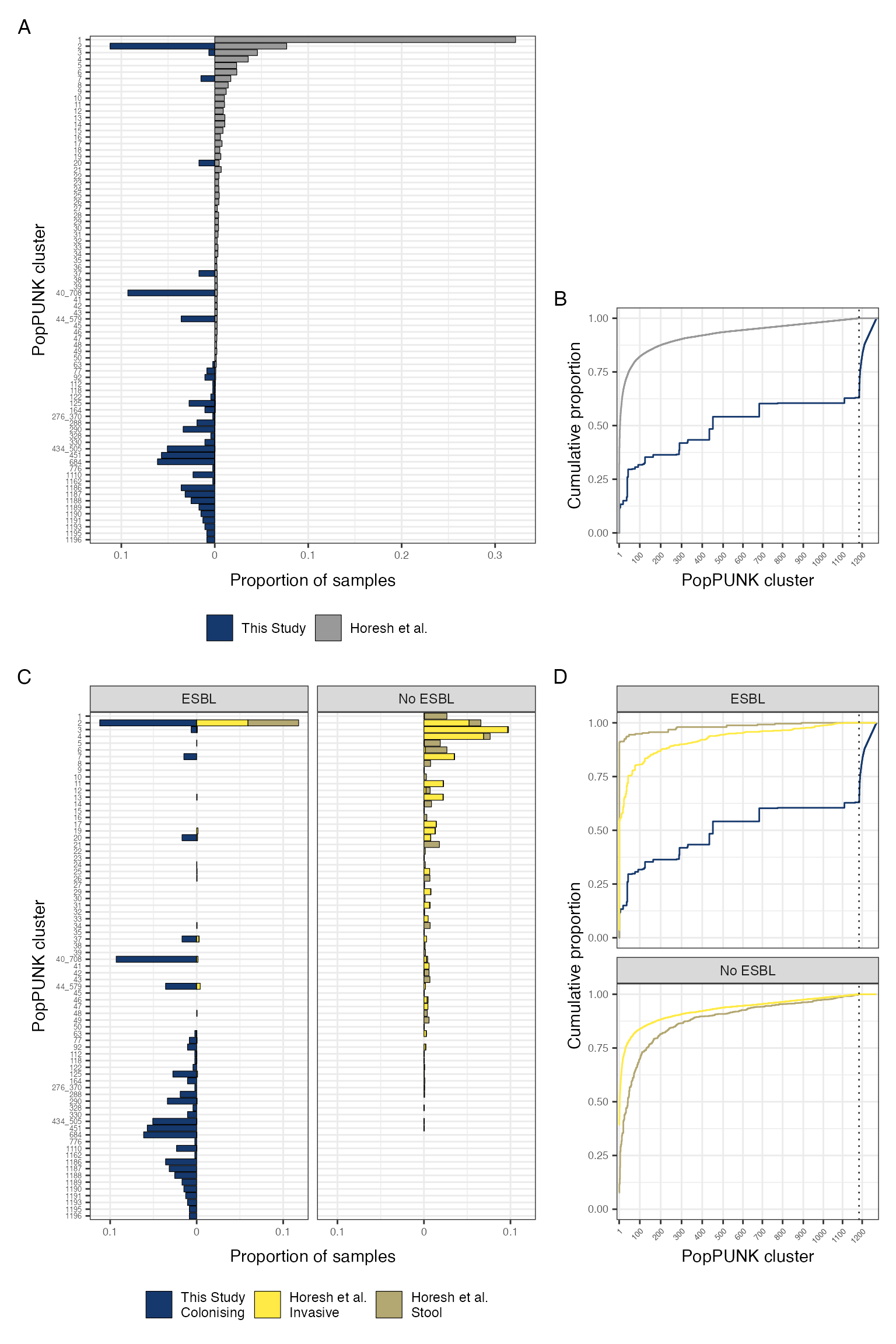
PopPUNK cluster assignments of isolates from this study, using the Horesh et al database. A: Proportion of samples assigned to a given cluster for this study (left) and the Horesh collection (right); clusters are ordered numerically which by definition is form largest to smallest in the Horesh collection. B: Cumulative proportion of isolates with cluster membership, with clusters again ordered numerically (i.e. largest to smallest). Dotted line indicates the end of clusters defined in the original Horesh popPUNK database; clusters to the right of this line are newly defined in the isolates in this study. C-E: The same plots but restricted to samples for which metadata on source of isolation is available (n = 3921) and stratfied by source and presence of absence of ESBL gene. Isolates with an identifiable ampC or carbapenemase gene are included in this category.
if (write_figs) {
  ggsave(
    here("figures/ecoli-genomics/global_poppunk_clusterplot_strat.pdf"),
    pp_cluster_plots_stratified,
    width = 8,
    height = 12
  )
  ggsave(
    here("figures/ecoli-genomics/global_poppunk_clusterplot_strat.svg"),
    pp_cluster_plots_stratified,
    width = 8,
    height = 12
  )
}
df_all %>%
  filter(study %in% c("dassim", "horesh")) %>%
  group_by(study, Cluster, ST) %>%
  summarise(n_ST = n()) %>%
  group_by(study, Cluster) %>%
  mutate(n_cluster = sum(n_ST))  %>%
  summarise(
    cluster_size = n_cluster,
            STprop = n_ST/n_cluster,
            STpropstr =
              paste0("ST", ST," (",
              formatC(n_ST / n_cluster, 2, format = "f"), ")"),
    )  ->
  df_clusttab
#> `summarise()` has grouped output by 'study', 'Cluster'. You can override using
#> the `.groups` argument.
#> Warning: Returning more (or less) than 1 row per `summarise()` group was deprecated in
#> dplyr 1.1.0.
#> ℹ Please use `reframe()` instead.
#> ℹ When switching from `summarise()` to `reframe()`, remember that `reframe()`
#>   always returns an ungrouped data frame and adjust accordingly.
#> Call `lifecycle::last_lifecycle_warnings()` to see where this warning was
#> generated.
#> `summarise()` has grouped output by 'study', 'Cluster'. You can override using
#> the `.groups` argument.

df_clusttab$STpropstr <-
  factor(df_clusttab$STpropstr, levels = unique(
    df_clusttab$STpropstr[order(df_clusttab$STprop,
                                decreasing = TRUE)])
    )

df_clusttab %>%
  filter(STprop >= 0.01) %>%
  pivot_wider(
    id_cols = c(Cluster),
   names_from = study,
   values_from = c(cluster_size,STpropstr),
   values_fn = list( STpropstr = function(x) paste(sort(x),collapse = ";"),
                     cluster_size = unique),
   values_fill = list(STpropstr = "-",
                      cluster_size = 0)
     ) %>%
  arrange(desc(cluster_size_dassim), desc(cluster_size_horesh)) %>%
  filter(cluster_size_dassim > 0) %>%
  left_join(
    df_all %>%
    filter(study %in% c("dassim", "horesh")) %>%
    group_by(Cluster) %>%
    summarise(pgroup = names(sort(table(Phylogroup), decreasing=TRUE)[1]))
  ) ->
  df_clusttab
#> Joining with `by = join_by(Cluster)`


df_all %>%
  filter(study %in% c("dassim", "horesh")) %>%
  group_by(study, Cluster, Continent) %>%
  summarise(n_continent = n()) %>%
  group_by(study, Cluster) %>%
  mutate(n_cluster = sum(n_continent))  %>%
  summarise(
    cluster_size = n_cluster,
            contprop = n_continent/n_cluster,
            contpropstr =
              paste0( Continent," (",
              formatC(n_continent / n_cluster, 2, format = "f"), ")"),
    )  ->
  df_clust.cont
#> `summarise()` has grouped output by 'study', 'Cluster'. You can override using
#> the `.groups` argument.
#> Warning: Returning more (or less) than 1 row per `summarise()` group was deprecated in
#> dplyr 1.1.0.
#> ℹ Please use `reframe()` instead.
#> ℹ When switching from `summarise()` to `reframe()`, remember that `reframe()`
#>   always returns an ungrouped data frame and adjust accordingly.
#> Call `lifecycle::last_lifecycle_warnings()` to see where this warning was
#> generated.
#> `summarise()` has grouped output by 'study', 'Cluster'. You can override using
#> the `.groups` argument.

df_clust.cont$contpropstr <-
  factor(df_clust.cont$contpropstr, levels = unique(
    df_clust.cont$contpropstr[order(df_clust.cont$contprop,
                                decreasing = TRUE)])
    )

left_join(df_clusttab,
df_clust.cont %>%
  pivot_wider(
    id_cols = c(Cluster),
   names_from = study,
   values_from = contpropstr,
   values_fn = function(x) paste(sort(x),collapse = ";"),
   values_fill = "-",
  )
) %>%
  arrange(desc(cluster_size_dassim), desc(cluster_size_horesh)) ->
  df_clusttab
#> Joining with `by = join_by(Cluster)`

df_all %>%
  filter(study %in% c("dassim", "horesh")) %>%
  mutate(Pathotype = gsub(" \\(predicted\\)","", Pathotype)) %>%
  group_by(study, Cluster, Pathotype) %>%
  summarise(n_path = n()) %>%
  group_by(study, Cluster) %>%
  mutate(n_cluster = sum(n_path))  %>%
  summarise(
    cluster_size = n_cluster,
            pathprop = n_path/n_cluster,
            pathpropstr =
              paste0( Pathotype," (",
              formatC(n_path / n_cluster, 2, format = "f"), ")"),
    )  ->
  df_clust.path
#> `summarise()` has grouped output by 'study', 'Cluster'. You can override using
#> the `.groups` argument.
#> Warning: Returning more (or less) than 1 row per `summarise()` group was deprecated in
#> dplyr 1.1.0.
#> ℹ Please use `reframe()` instead.
#> ℹ When switching from `summarise()` to `reframe()`, remember that `reframe()`
#>   always returns an ungrouped data frame and adjust accordingly.
#> Call `lifecycle::last_lifecycle_warnings()` to see where this warning was
#> generated.
#> `summarise()` has grouped output by 'study', 'Cluster'. You can override using
#> the `.groups` argument.

df_clust.path$pathpropstr <-
  factor(df_clust.path$pathpropstr, levels = unique(
    df_clust.path$pathpropstr[order(df_clust.path$pathprop,
                                decreasing = TRUE)])
    )


left_join(df_clusttab,
df_clust.path %>%
  pivot_wider(
    id_cols = c(Cluster),
   names_from = study,
   values_from = pathpropstr,
   values_fn = function(x) paste(sort(x),collapse = ";"),
   values_fill = "-",
  ) %>%
  transmute(
    Cluster = Cluster,
    horesh_pathotype = horesh,
)) ->
  df_clusttab
#> Joining with `by = join_by(Cluster)`


df_clusttab %>%
  select(Cluster,
         pgroup,
         cluster_size_dassim,
         STpropstr_dassim,
         cluster_size_horesh,
         STpropstr_horesh,
         horesh,
         horesh_pathotype
         ) %>%
  kbl(caption =
        "Cluster assigment of samples from this study compared to Horesh collection",
      col.names = c("Cluster","Phylogroup",
                    rep(c(
                    "n isolates",
                    "STs"),2),"Location", "Pathotype")
      ) %>%
  kable_classic(full_width = FALSE) %>%
add_header_above(c(" " = 2, "This Study" = 2, "Horesh Collection" = 4))|
This Study
|
Horesh Collection
|
||||||
|---|---|---|---|---|---|---|---|
| Cluster | Phylogroup | n isolates | STs | n isolates | STs | Location | Pathotype |
| 2 | B2 | 53 | ST131 (1.00) | 781 | ST131 (0.99) | Europe (0.73);Unknown (0.12);Americas (0.11);Oceania (0.03);Asia (0.00) | ExPEC (0.54);Not determined (0.46) |
| 40_708 | C | 44 | ST410 (1.00) | 29 | ST23 (0.41);ST410 (0.34);ST2230 (0.07);ST369 (0.07);ST5491 (0.07);ST5286 (0.03) | Europe (0.62);Americas (0.31);Asia (0.07) | ExPEC (0.55);STEC (0.21);ETEC (0.17);Not determined (0.07) |
| 684 | A | 29 | ST44 (1.00) | 1 | ST44 (1.00) | Europe (1.00) | ExPEC (1.00) |
| 451 | B2 | 27 | ST636 (1.00) | 1 | ST636 (1.00) | Americas (1.00) | ExPEC (1.00) |
| 434_505 | A | 24 | ST167 (0.92);ST10 (0.08) | 3 | ST10 (1.00) | Americas (0.67);Europe (0.33) | ExPEC (0.67);Not determined (0.33) |
| 44_579 | F | 17 | ST648 (1.00) | 26 | ST648 (1.00) | Europe (0.42);Unknown (0.38);Americas (0.19) | ExPEC (0.73);Not determined (0.27) |
| 1186 | A | 17 | ST656 (1.00) | 0 |
|
|
|
| 290 | A | 16 | ST46 (1.00) | 2 | ST46 (1.00) | Americas (1.00) | ExPEC (0.50);Not determined (0.50) |
| 1187 | B1 | 15 | ST940 (1.00) | 0 |
|
|
|
| 125 | A | 13 | ST617 (0.92);ST4981 (0.08) | 7 | ST617 (1.00) | Americas (0.71);Europe (0.29) | ExPEC (0.57);Not determined (0.43) |
| 1188 | A | 12 | ST167 (1.00) | 0 |
|
|
|
| 1110 | F | 11 | ST1722 (1.00) | 1 | ST1722 (1.00) | Europe (1.00) | ExPEC (1.00) |
| 288 | A | 9 | ST5824 (1.00) | 3 | ST227 (1.00) | Americas (1.00) | Not determined (1.00) |
| 20 | B2 | 8 | ST131 (1.00) | 48 | ST131 (0.96);ST5432 (0.02);ST5494 (0.02) | Europe (0.75);Americas (0.12);Unknown (0.10);Oceania (0.02) | ExPEC (0.71);Not determined (0.29) |
| 37 | D | 8 | ST405 (1.00) | 27 | ST405 (0.96);ST964 (0.04) | Europe (0.63);Americas (0.33);Asia (0.04) | ExPEC (0.81);Not determined (0.11);ETEC (0.04);STEC (0.04) |
| 1189 | A | 8 | ST1421 (1.00) | 0 |
|
|
|
| 7 | D | 7 | ST69 (1.00) | 174 | ST69 (0.94);ST106 (0.03) | Europe (0.83);Americas (0.12);Unknown (0.05) | ExPEC (0.79);Not determined (0.19);EAEC (0.02) |
| 1190 | A | 7 | ST9847 (1.00) | 0 |
|
|
|
| 1191 | D | 6 | ST38 (0.83);STNovel (0.17) | 0 |
|
|
|
| 92 | A | 5 | ST10 (1.00) | 10 | ST10 (1.00) | Europe (0.60);Americas (0.40) | ExPEC (0.60);Not determined (0.40) |
| 164 | A | 5 | ST34 (1.00) | 6 | ST34 (1.00) | Africa (0.67);Europe (0.33) | EPEC (0.67);Not determined (0.33) |
| 330 | B1 | 5 | ST101 (1.00) | 2 | ST101 (1.00) | Europe (0.50);Unknown (0.50) | Not determined (1.00) |
| 1193 | A | 5 | ST10 (1.00) | 0 |
|
|
|
| 77 | D | 4 | ST38 (1.00) | 11 | ST38 (0.73);ST315 (0.27) | Europe (1.00) | Not determined (0.82);ExPEC (0.18) |
| 1195 | D | 4 | ST6636 (1.00) | 0 |
|
|
|
| 1196 | D | 4 | ST38 (1.00) | 0 |
|
|
|
| 3 | B2 | 3 | ST73 (1.00) | 463 | ST73 (0.94);ST104 (0.01) | Europe (0.85);Americas (0.11);Unknown (0.03);Asia (0.00);Africa (0.00) | ExPEC (0.83);Not determined (0.16);STEC (0.01);EAEC (0.00) |
| 1194 | A | 3 | ST48 (1.00) | 0 |
|
|
|
| 1197 | F | 3 | ST354 (1.00) | 0 |
|
|
|
| 1198 | B1 | 3 | ST517 (1.00) | 0 |
|
|
|
| 1199 | F | 3 | ST354 (1.00) | 0 |
|
|
|
| 1200 | A | 3 | ST617 (1.00) | 0 |
|
|
|
| 1201 | A | 3 | ST46 (1.00) | 0 |
|
|
|
| 1202 | A | 3 | ST10 (1.00) | 0 |
|
|
|
| 122 | B1 | 2 | ST443 (1.00) | 6 | ST443 (1.00) | Europe (0.83);Asia (0.17) | Not determined (0.67);EPEC (0.17);ExPEC (0.17) |
| 328 | B1 | 2 | ST224 (1.00) | 2 | ST224 (1.00) | Americas (1.00) | ExPEC (0.50);Not determined (0.50) |
| 1205 | A | 2 | ST617 (1.00) | 0 |
|
|
|
| 1206 | A | 2 | ST3168 (1.00) | 0 |
|
|
|
| 1207 | A | 2 | ST2705 (1.00) | 0 |
|
|
|
| 1208 | B1 | 2 | ST424 (1.00) | 0 |
|
|
|
| 1209 | E | 2 | ST219 (1.00) | 0 |
|
|
|
| 1210 | F | 2 | ST1722 (1.00) | 0 |
|
|
|
| 1211 | A | 2 | ST1201 (1.00) | 0 |
|
|
|
| 1212 | A | 2 | ST617 (1.00) | 0 |
|
|
|
| 1213 | A | 2 | ST48 (1.00) | 0 |
|
|
|
| 63 | D | 1 | ST38 (1.00) | 17 | ST38 (0.94);ST778 (0.06) | Europe (0.59);Unknown (0.18);Americas (0.18);Asia (0.06) | Not determined (0.53);ExPEC (0.47) |
| 112 | A | 1 | ST2089 (1.00) | 7 | ST2089 (1.00) | Europe (0.71);Africa (0.14);Asia (0.14) | Not determined (0.71);EPEC (0.29) |
| 118 | A | 1 | ST167 (1.00) | 6 | ST167 (1.00) | Europe (1.00) | Not determined (0.67);ExPEC (0.33) |
| 276_370 | B1 | 1 | ST156 (1.00) | 3 | ST156 (0.67);ST348 (0.33) | Americas (0.33);Europe (0.33);Asia (0.33) | Not determined (0.67);ExPEC (0.33) |
| 1162 | B1 | 1 | ST224 (1.00) | 1 | ST224 (1.00) | Europe (1.00) | Not determined (1.00) |
| 776 | F | 1 | ST1485 (1.00) | 1 | ST1485 (1.00) | Europe (1.00) | Not determined (1.00) |
| 1192 | D | 1 | ST391 (1.00) | 0 |
|
|
|
| 1235 | A | 1 | ST1237 (1.00) | 0 |
|
|
|
| 1236 | A | 1 | ST3489 (1.00) | 0 |
|
|
|
| 1237 | A | 1 | ST4981 (1.00) | 0 |
|
|
|
| 1238 | B1 | 1 | ST3580 (1.00) | 0 |
|
|
|
| 1239 | F | 1 | ST648 (1.00) | 0 |
|
|
|
| 1240 | A | 1 | ST48 (1.00) | 0 |
|
|
|
| 1241 | Unknown | 1 | ST167 (1.00) | 0 |
|
|
|
| 1242 | A | 1 | ST191 (1.00) | 0 |
|
|
|
| 1243 | B1 | 1 | ST2083 (1.00) | 0 |
|
|
|
| 1244 | A | 1 | ST48 (1.00) | 0 |
|
|
|
| 1245 | B1 | 1 | ST2077 (1.00) | 0 |
|
|
|
| 1246 | B1 | 1 | ST2852 (1.00) | 0 |
|
|
|
| 1247 | A | 1 | ST44 (1.00) | 0 |
|
|
|
| 1248 | Unknown | 1 | ST410 (1.00) | 0 |
|
|
|
| 1249 | Unknown | 1 | ST44 (1.00) | 0 |
|
|
|
| 1250 | A | 1 | ST617 (1.00) | 0 |
|
|
|
| 1251 | D | 1 | ST38 (1.00) | 0 |
|
|
|
| 1252 | B2 | 1 | ST131 (1.00) | 0 |
|
|
|
| 1253 | B1 | 1 | ST1081 (1.00) | 0 |
|
|
|
| 1254 | E | 1 | ST1944 (1.00) | 0 |
|
|
|
| 1255 | A | 1 | STNovel (1.00) | 0 |
|
|
|
| 1256 | Unknown | 1 | ST617 (1.00) | 0 |
|
|
|
| 1257 | A | 1 | ST10 (1.00) | 0 |
|
|
|
| 1258 | A | 1 | STNovel (1.00) | 0 |
|
|
|
| 1259 | Unknown | 1 | ST131 (1.00) | 0 |
|
|
|
| 1260 | A | 1 | ST226 (1.00) | 0 |
|
|
|
| 1261 | D | 1 | ST38 (1.00) | 0 |
|
|
|
| 1262 | A | 1 | ST10 (1.00) | 0 |
|
|
|
| 1263 | B1 | 1 | ST155 (1.00) | 0 |
|
|
|
| 1264 | A | 1 | ST617 (1.00) | 0 |
|
|
|
| 1265 | A | 1 | STNovel (1.00) | 0 |
|
|
|
| 1266 | D | 1 | ST349 (1.00) | 0 |
|
|
|
| 1267 | F | 1 | ST354 (1.00) | 0 |
|
|
|
| 1268 | A | 1 | ST167 (1.00) | 0 |
|
|
|
| 1269 | Unknown | 1 | STNovel (1.00) | 0 |
|
|
|
| 1270 | A | 1 | ST1421 (1.00) | 0 |
|
|
|
| 1271 | B1 | 1 | ST155 (1.00) | 0 |
|
|
|
| 1272 | A | 1 | ST609 (1.00) | 0 |
|
|
|
| 1273 | B2 | 1 | ST131 (1.00) | 0 |
|
|
|
| 1274 | D | 1 | ST405 (1.00) | 0 |
|
|
|
| 1275 | B1 | 1 | ST155 (1.00) | 0 |
|
|
|
| 1276 | B1 | 1 | ST906 (1.00) | 0 |
|
|
|
| 1277 | A | 1 | ST617 (1.00) | 0 |
|
|
|
| 1278 | Unknown | 1 | ST167 (1.00) | 0 |
|
|
|
| 1279 | A | 1 | ST48 (1.00) | 0 |
|
|
|
| 1280 | A | 1 | ST1303 (1.00) | 0 |
|
|
|
| 1281 | A | 1 | ST6438 (1.00) | 0 |
|
|
|
| 1282 | A | 1 | ST206 (1.00) | 0 |
|
|
|
| 1283 | B1 | 1 | ST1146 (1.00) | 0 |
|
|
|
| 1284 | B1 | 1 | ST46 (1.00) | 0 |
|
|
|
| 1285 | A | 1 | ST401 (1.00) | 0 |
|
|
|
| 1286 | A | 1 | ST44 (1.00) | 0 |
|
|
|
| 1287 | A | 1 | ST10 (1.00) | 0 |
|
|
|
| 1288 | Unknown | 1 | ST48 (1.00) | 0 |
|
|
|
| 1289 | B1 | 1 | ST155 (1.00) | 0 |
|
|
|
| 1290 | Unknown | 1 | ST10 (1.00) | 0 |
|
|
|
| 1291 | A | 1 | ST3856 (1.00) | 0 |
|
|
|
if (write_figs) {
 write_csv(df_clusttab %>%
             transmute(
               Cluster = Cluster,
               Phylogroup = pgroup,
               n_this_study = cluster_size_dassim,
               STs_this_study = STpropstr_dassim,
               n_horesh = cluster_size_horesh,
               STs_horesh = STpropstr_horesh,
               location_horesh = horesh,
               pathotype_horesh = horesh_pathotype),
           here("tables/ecoli-genomics/cluster_stats.csv")
 )

}
# bits and bobs to calculate for manuscript

# how many clusters?

dassimEcoli_BTEcoli.accession %>%
  group_by(Cluster) %>%
  tally() %>%
  nrow()
#> [1] 87

dassimEcoli_BTEcoli.accession %>%
  group_by(Cluster) %>%
  tally() %>%
  summarise(
    median_size = median(n),
    lq = quantile(n, 0.25),
    uq = quantile(n, 0.75)
  )
#> # A tibble: 1 × 3
#>   median_size    lq    uq
#>         <int> <dbl> <dbl>
#> 1           1     1     5


dassimEcoli_BTEcoli.accession %>%
  group_by(Cluster) %>%
  tally() %>%
  arrange(-n)
#> # A tibble: 87 × 2
#>    Cluster     n
#>    <chr>   <int>
#>  1 E1         53
#>  2 E2         46
#>  3 E3         45
#>  4 E4         33
#>  5 E5         27
#>  6 E6         22
#>  7 E7         18
#>  8 E8         17
#>  9 E9         16
#> 10 E10        15
#> # ℹ 77 more rows

dassimEcoli_BTEcoli.accession %>%
  group_by(Cluster, ST) %>%
  tally() %>%
  arrange(-n)
#> # A tibble: 92 × 3
#> # Groups:   Cluster [87]
#>    Cluster ST        n
#>    <chr>   <chr> <int>
#>  1 E1      131      53
#>  2 E3      410      45
#>  3 E2      167      36
#>  4 E4      44       32
#>  5 E5      636      27
#>  6 E6      617      21
#>  7 E7      648      18
#>  8 E8      656      17
#>  9 E9      46       16
#> 10 E10     940      15
#> # ℹ 82 more rows

df_all %>%
  filter(study == "dassim") %>%
  mutate(numeric_cluster = as.numeric(
    gsub("_.*$","",Cluster)),
    clust_50orbelow =
           case_when(
             numeric_cluster <= 50 ~ "top 50",
             numeric_cluster <=1184 ~ "not top 50 but in horsh cluster",
             TRUE ~ "new cluster")
  ) %>%
  group_by(clust_50orbelow) %>%
  tally() %>%
  mutate(
    tot = sum(n),
    prop = n/sum(n))
#> # A tibble: 3 × 4
#>   clust_50orbelow                     n   tot  prop
#>   <chr>                           <int> <int> <dbl>
#> 1 new cluster                       175   473 0.370
#> 2 not top 50 but in horsh cluster   158   473 0.334
#> 3 top 50                            140   473 0.296

btESBL_ecoli_horesh_metadata %>%
  mutate(clust_50orbelow =
           case_when(
             PopPUNK <= 50 ~ "top 50",
             PopPUNK <=1184 ~ "not top 50 but in horsh cluster",
             TRUE ~ "new cluster")
         ) %>%
  group_by(clust_50orbelow) %>%
  tally() %>%
  mutate(
    tot = sum(n),
    prop = n/sum(n))
#> # A tibble: 2 × 4
#>   clust_50orbelow                     n   tot  prop
#>   <chr>                           <int> <int> <dbl>
#> 1 not top 50 but in horsh cluster  2459 10146 0.242
#> 2 top 50                           7687 10146 0.758

amr %>%
  select(lane, class) %>%
  unique() %>%
  ungroup() %>%
  mutate(n_tot = length(unique(lane))) %>%
  group_by(class) %>%
  summarise(n = n(),
            n_tot = max(n_tot),
            prop = n/n_tot
  )
#> # A tibble: 14 × 4
#>    class               n n_tot    prop
#>    <chr>           <int> <int>   <dbl>
#>  1 Aminoglycoside    469   473 0.992
#>  2 AmpC               45   473 0.0951
#>  3 Carbapenemase       1   473 0.00211
#>  4 Chloramphenicol   248   473 0.524
#>  5 ESBL              472   473 0.998
#>  6 Fosfomycin         28   473 0.0592
#>  7 Macrolide         325   473 0.687
#>  8 Penicillinase     347   473 0.734
#>  9 Quinolone         407   473 0.860
#> 10 Rifampicin          2   473 0.00423
#> 11 Streptothricin     69   473 0.146
#> 12 Sulphonamide      468   473 0.989
#> 13 Tetracycline      411   473 0.869
#> 14 Trimethoprim      459   473 0.970


  df_all %>%
    filter(study == "dassim", ST != "Novel") %>%
    group_by(ST) %>%
    summarise(n = n()) %>%
    ungroup() %>%
    summarise(
      m = median(n),
      min = min(n),
      lq = quantile(n, 0.25),
      uq = quantile(n, 0.75),
      max = max(n)
    )
#> # A tibble: 1 × 5
#>       m   min    lq    uq   max
#>   <int> <int> <dbl> <dbl> <int>
#> 1     2     1     1     9    64

  #QRDR stuff

  btESBL_amrgenes %>%
  semi_join(dassimEcoli_BTEcoli.accession,
            by = c( "lane")) %>%
  select(-genus) %>%
  rename(gene = ref_seq) %>%
  # add in QRDR mutations
  bind_rows(
    btESBL_qrdr_mutations %>%
      filter(genus == "E. coli") %>%
      select(-genus) %>%
      semi_join(
        btESBL_CARD_qrdr_mutations,
        by = c("variant" = "variant",
              "gene" =  "gene")
      ) %>%
      unique() %>%
      mutate(gene =
               gsub("(^.{1})", '\\U\\1',
                    gene,
                    perl = TRUE))
      ) %>%
  filter(!grepl("AmpH|AMPH|AmpC|MrdA|MefB", gene)) %>%
  # add in beta-lactamases
  left_join(
    select(btESBL_NCBI_phenotypic_bl, allele_name, class),
    by = c("gene" = "allele_name")) %>%
  mutate(class = case_when(
    str_detect(gene, quinolone) ~ "Quinolone",
    str_detect(gene, tetracycline) ~ "Tetracycline",
    str_detect(gene, sulphonamide) ~ "Sulphonamide",
    str_detect(gene, aminoglycoside) ~ "Aminoglycoside",
    str_detect(gene, streptothricin) ~ "Streptothricin",
    str_detect(gene, macrolide) ~ "Macrolide",
    str_detect(gene, fosfomycin) ~ "Fosfomycin",
    str_detect(gene, chloramphenicol) ~ "Chloramphenicol",
    str_detect(gene, rifampicin) ~ "Rifampicin",
    str_detect(gene,trimethoprim) ~ "Trimethoprim",
    str_detect(gene,ESBL) ~ "ESBL",
    str_detect(gene,penicillinase) ~ "Penicillinase",
    str_detect(gene,ampc) ~ "AmpC",
    TRUE ~ class
  )) %>%
    filter(class == "Quinolone") -> quinolone.amr

  quinolone.amr %>%
    mutate(gene = paste0(gene,
                         if_else(
                           !is.na(variant),
                           variant, ""))) %>%
    select(lane,gene) %>%
    unique() %>%
    pivot_wider(id_cols = lane,
                names_from = gene,
                values_from = gene,
                values_fn = length,
                values_fill = 0) %>%
    summarise(across(!contains("lane"), sum))
#> # A tibble: 1 × 10
#>    QepA Qnr_S1 QnrB19 QnrS2 QnrB6 QnrB1 GyrAS83L GyrAD87N ParCS80I ParCE84G
#>   <int>  <int>  <int> <int> <int> <int>    <int>    <int>    <int>    <int>
#> 1    47     57      2     1     2     2      351      294      296        8


quinolone.amr %>%
  group_by(lane) %>%
  summarise(qrdr = any(grepl("Gyr|Par", gene)),
            qnr = any(grepl("Qnr", gene)),
            qep = any(grepl("Qep", gene))) %>%
  ungroup() %>%
  summarise(qrdr_alone = sum(qrdr & !qnr & !qep),
            qnr_alone = sum(qnr & !qrdr & !qep),
            qrdr_qnr = sum(qrdr & qnr),
            qrdr_qep = sum(qrdr & qep),
            qnr_qep = sum(qnr & qep)
  )
#> # A tibble: 1 × 5
#>   qrdr_alone qnr_alone qrdr_qnr qrdr_qep qnr_qep
#>        <int>     <int>    <int>    <int>   <int>
#> 1        299        56        6       47       1
btESBL_plasmidreplicons %>%
  filter(species == "E. coli") %>%
   mutate(ref_seq = gsub("_.+$","", ref_seq),
         ref_seq = gsub("\\.[0-9]","", ref_seq),
         ref_seq = case_when(
           grepl("Col", ref_seq) ~ "Col",
           grepl("rep", ref_seq) ~ "rep",
           grepl("^FIA", ref_seq) ~ "IncFIA",
           !grepl("Inc", ref_seq) ~ "Other",
           TRUE ~ ref_seq
          )) %>%
  filter(grepl("Inc", ref_seq)) %>%
  arrange(fct_infreq(ref_seq)) %>%
  pivot_wider(id_cols = lane,
              values_from = ref_seq,
              names_from = ref_seq,
              values_fn = length,
              values_fill = 0) %>%
  mutate(across(where(is.numeric), ~ if_else(.x >= 1, "Present", "Absent"))) %>%
  as.data.frame() ->
  btESBL_plasmidreplicons_onehot

rownames(btESBL_plasmidreplicons_onehot) <- btESBL_plasmidreplicons_onehot$lane


ggtree(btESBL_coregene_tree_esco) %>%
  gheatmap(select(btESBL_plasmidreplicons_onehot, -lane),
           font.size = 2.5,
           color = NA,
           colnames_angle = 90,
           offset = 0,
           colnames_offset_y = 3,
           colnames_position = "top",
           hjust = 0) +
  ylim(NA,550) +
  labs(fill = "Plasmid\nReplicon") +
  scale_fill_manual(values = c("white", "darkgrey"),
                     na.translate = FALSE) -> plas_replicons_map_to_tree
#> Scale for y is already present.
#> Adding another scale for y, which will replace the existing scale.
#> Scale for fill is already present.
#> Adding another scale for fill, which will replace the existing scale.
  plas_replicons_map_to_tree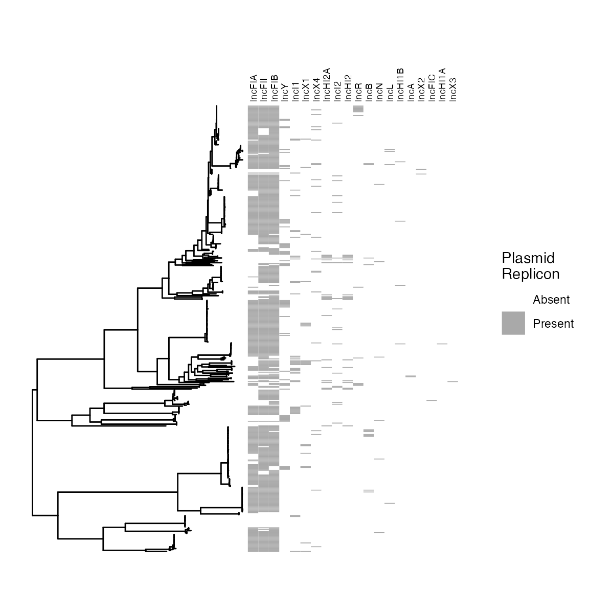
Plasmid replicons mapped back to tree
ST410 trees
btESBL_ecoli_st410_metadata %>%
  filter(accession %in% btESBL_ecoli_globalst410_tree$tip.label) %>%
  bind_rows(
    btESBL_sequence_sample_metadata %>%
      filter(lane %in% btESBL_ecoli_globalst410_tree$tip.label) %>%
      transmute(accession = lane,
                `Collection Year` = year(data_date),
                host = "Homo sapiens",
                source = "Stool",
                Country = "Malawi")
  ) %>%
  rename(
    Year = `Collection Year`) %>%
  as.data.frame() -> st410_metadata

if (write_figs) {
st410_metadata %>%
  filter(Country != "Malawi") %>%
  transmute(accession = accession,
            country = Country,
            year = Year) %>%
  write_csv(here("tables/ecoli-genomics/SUPP_T_st410_accession_numbers_and_metadata.csv"))
}

st410_metadata$malawi <- st410_metadata$Country == "Malawi"


st410_metadata$Continent <-
  countrycode(
    sourcevar = st410_metadata$Country,
    origin = "country.name",
    destination = "un.region.name"
  )
#> Warning: Some values were not matched unambiguously: -, Africa, Asia, Blantyre, Europe

st410_metadata %>%
  mutate(
    Continent = case_when(
      Country %in% c("Africa", "Asia", "Europe") ~
      Country,
      Country == "Blantyre" ~ "Africa",
      TRUE ~ Continent
    )
  ) ->
st410_metadata

rownames(st410_metadata) <- st410_metadata$accession


btESBL_ecoli_st410_amr %>%
  pivot_wider(
    names_from = gene,
    values_from = gene,
    values_fn = length,
    values_fill = 0
  ) %>%
  mutate(across(everything(), as.character)) %>%
  as.data.frame() ->
amr.ariba410


rownames(amr.ariba410) <- amr.ariba410$name


btESBL_ecoli_st410_amr %>%
  bind_rows(
    btESBL_amrgenes %>%
      filter(genus == "E. coli") %>%
      select(-genus) %>%
      transmute(
        name = lane,
        gene = ref_seq
      )
  ) %>%
  filter(name %in% btESBL_ecoli_globalst410_tree$tip.label) %>%
  left_join(
    select(btESBL_NCBI_phenotypic_bl, allele_name, class),
    by = c("gene" = "allele_name")
  ) %>%
  mutate(class = case_when(
    grepl("CMY", name) ~ "ESBL/AmpC",
    class == "ESBL" ~ "ESBL/AmpC",
    TRUE ~ class
  )) %>%
  filter(class %in% c("ESBL/AmpC", "Carbapenemase")) %>%
  mutate(gene = gsub("_", "-", gene)) %>%
  arrange(class, fct_infreq(gene)) %>%
  pivot_wider(
    id_cols = "name",
    names_from = gene,
    values_from = class
  ) %>%
  as.data.frame() ->
esbl_cpe.ariba410
rownames(esbl_cpe.ariba410) <- esbl_cpe.ariba410$name

btESBL_ecoli_st410_plasmids %>%
  bind_rows(
    btESBL_plasmidreplicons %>%
      mutate(
        ref_seq = gsub("\\..*$", "", ref_seq),
        ref_seq = gsub("_.*$", "", ref_seq),
        ref_seq = gsub("^FIA", "IncFIA", ref_seq)
      ) %>%
      filter(species == "E. coli") %>%
      select(-species) %>%
      rename(name = lane)
  ) %>%
  filter(name %in% btESBL_ecoli_globalst410_tree$tip.label) %>%
  filter(grepl("Inc", ref_seq)) %>%
  unique() %>%
  arrange(fct_infreq(ref_seq)) %>%
  pivot_wider(
    id_cols = name,
    names_from = ref_seq,
    values_from = ref_seq,
    values_fn = function(x) {
      return("Present")
    },
    values_fill = NA_character_
  ) %>%
  as.data.frame() -> st410_plasm_onehot
rownames(st410_plasm_onehot) <- st410_plasm_onehot$name


(
(
  (ggtree(
    btESBL_ecoli_globalst410_tree) %<+%
     (select(st410_metadata, accession, Country) %>%
        mutate(Country = if_else(Country == "Malawi", "Malawi",NA_character_)))  %>%
     gheatmap(
       select(st410_metadata, `Year`),
       font.size = 4,
       width = 0.03,
       colnames_position = "top",
       color = NA,
       colnames_offset_y = 5,
       colnames_angle = 90,
       hjust = 0
     )  +
     scale_fill_viridis(name = "Year", na.value = "white") +
     new_scale_fill()) %>%
  gheatmap(
    select(st410_metadata, Continent),
    font.size = 4,
    width = 0.03,
    colnames_position = "top",
    color = NA,
    colnames_offset_y = 5,
    colnames_angle = 90,
    offset = 0.000008,
    hjust = 0
  ) +
  scale_fill_viridis_d(option = "plasma", name = "Continent", na.translate =
                       FALSE) +
  geom_tippoint(aes(color = Country), na.rm = TRUE, size = 0.5) +
  scale_color_manual(values  = "red", na.translate = FALSE) +
  new_scale_fill()
) %>%
  gheatmap(
    select(esbl_cpe.ariba410, -name),
    font.size = 3,
    width = 0.6,
    colnames_position = "top",
    color = NA,
    colnames_offset_y = 5,
    colnames_angle = 90,
    offset = 0.000016,
    hjust = 0
  ) + scale_fill_manual(values = viridis_pal(option = "magma")(5)[c(2,3)],
                        na.translate = FALSE,
                        name = "Beta-\nlactamase") +
  new_scale_fill()
) + # %>%
  # gheatmap(
  #   select(st410_plasm_onehot, -name),
  #   font.size = 3,
  #   width = 0.5,
  #   colnames_position = "top",
  #   color = NA,
  #   colnames_offset_y = 5,
  #   colnames_angle = 90,
  #   offset = 0.0026,
  #   hjust = 0
  # ) + scale_fill_manual(values = viridis_pal(option = "cividis")(7)[2],
  #                       na.translate = FALSE,
  #                       name = "Plasmid\nreplicon") +
  ylim(NA, 420) +
  geom_treescale(x = 0.00005, y = 250, offset = 5) +
   geom_highlight(node = 391 ,alpha = 0.3) +
  geom_cladelabel(
    node = 391,
    label = "B4/H24RxC",
    angle = 90,
    offset = 0,
    offset.text = -0.000032,
    barsize = 0,
    hjust = 0.5,
    fontsize = 3,
    color = "steelblue"
  )  -> st410_globaltree_plot
#> Scale for fill is already present.
#> Adding another scale for fill, which will replace the existing scale.
#> Scale for fill is already present.
#> Adding another scale for fill, which will replace the existing scale.
#> Scale for fill is already present.
#> Adding another scale for fill, which will replace the existing scale.
#> Scale for y is already present.
#> Adding another scale for y, which will replace the existing scale.

if (write_figs) {

ggsave(here("figures/ecoli-genomics/st410_globaltreeplot.svg"),
       st410_globaltree_plot, width = 9, height = 10)

ggsave(here("figures/ecoli-genomics/st410_globaltreeplot.pdf"),
       st410_globaltree_plot, width = 9, height = 10)
}
st410_globaltree_plot
#> Warning: The following aesthetics were dropped during statistical transformation: node,
#> parent
#> ℹ This can happen when ggplot fails to infer the correct grouping structure in
#>   the data.
#> ℹ Did you forget to specify a `group` aesthetic or to convert a numerical
#>   variable into a factor?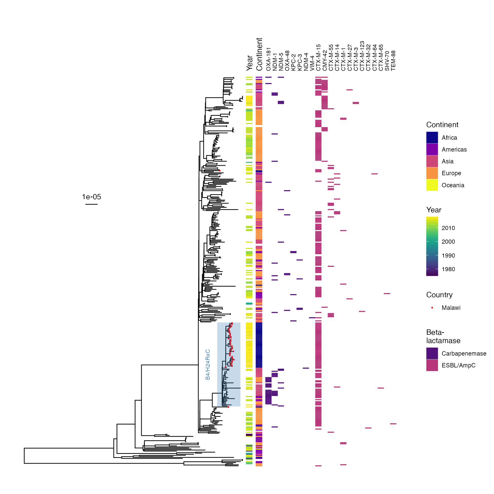
ST410 map-to-reference global maximum likelihood, midpoint rooted tree
tree_subset(
  btESBL_ecoli_globalst410_tree, 390, levels_back = 0)  -> st410_subtree

esbl_cpe.ariba410 %>%
  subset(name %in% st410_subtree$tip.label) %>%
  as.data.frame() ->
esbl_cpe.ariba410_subset

  esbl_cpe.ariba410_subset[
    c(TRUE, apply(esbl_cpe.ariba410_subset[-1], 2, function(x) !all(is.na(x))))
  ] ->
  esbl_cpe.ariba410_subset

btESBL_ecoli_st410_plasmids %>%
  bind_rows(
    btESBL_plasmidreplicons %>%
      mutate(
        ref_seq = gsub("\\..*$", "", ref_seq),
        ref_seq = gsub("_.*$", "", ref_seq),
        ref_seq = gsub("^FIA", "IncFIA", ref_seq)
      ) %>%
      filter(species == "E. coli") %>%
      select(-species) %>%
      rename(name = lane)
  ) %>%
  filter(grepl("Inc", ref_seq)) %>%
  filter(name %in% st410_subtree$tip.label) %>%
  unique() %>%
  group_by(ref_seq) %>%
  mutate(n = n()) %>%
  filter(n > 2) %>%
  ungroup() %>%
  select(-n) %>%
  arrange(fct_infreq(ref_seq)) %>%
  pivot_wider(
    id_cols = name,
    names_from = ref_seq,
    values_from = ref_seq,
    values_fn = function(x) {
      return("Present")
    },
    values_fill = NA_character_
  ) %>%
  as.data.frame() -> st410_plasm_onehot_subset
rownames(st410_plasm_onehot_subset) <- st410_plasm_onehot_subset$name

(
  (
    (ggtree(st410_subtree, size = 0.3) %<+% (select(st410_metadata, accession, Country) %>% mutate(Country = if_else(Country == "Malawi", "Malawi", NA_character_))) %>%
      gheatmap(
        select(st410_metadata, `Year`),
        font.size = 4,
        width = 0.06,
        colnames_position = "top",
        color = NA,
        colnames_offset_y = 0,
        colnames_angle = 90,
        hjust = 0
      ) +
      scale_fill_viridis(
        name = "Year", limits = c(1978, 2020),
        na.value = "white"
      ) +
      new_scale_fill()) %>%
      gheatmap(
        select(st410_metadata, Continent),
        font.size = 4,
        width = 0.06,
        colnames_position = "top",
        color = NA,
        colnames_offset_y = 0,
        colnames_angle = 90,
        offset = 0.0000015,
        hjust = 0
      ) +
      scale_fill_viridis_d(
        option = "plasma", name = "Continent",
        na.translate = FALSE
      ) +
      geom_point2(aes(subset = as.numeric(label) < 95 & !isTip), size = 0.5) +
      geom_tippoint(aes(color = Country), na.rm = TRUE, size = 1) +
      scale_color_manual(values = "red", na.translate = FALSE) +
      new_scale_fill()
  ) %>%
    gheatmap(
      select(esbl_cpe.ariba410_subset, -name),
      font.size = 2.5,
      width = 0.4,
      colnames_position = "top",
      color = NA,
      colnames_offset_y = 0,
      colnames_angle = 90,
      offset = 0.0000031,
      hjust = 0
    ) + scale_fill_manual(
      values = viridis_pal(option = "magma")(5)[c(2, 3)],
      na.translate = FALSE,
      name = "Beta-\nlactamase"
    ) +
    new_scale_fill()
) %>%
  gheatmap(
    select(st410_plasm_onehot_subset, -name),
    font.size = 2.5,
    width = 0.45,
    colnames_position = "top",
    color = NA,
    colnames_offset_y = 0,
    colnames_angle = 90,
    offset = 0.0000125,
    hjust = 0
  ) + scale_fill_manual(
    values = viridis_pal(option = "cividis")(7)[2],
    na.translate = FALSE,
    name = "Plasmid\nreplicon"
  ) +
  ylim(NA, 100) +
  geom_treescale(x = 0.000004, y = 66, offset = 2, width = 1e-6) ->
st410_subtree_plot
#> Scale for fill is already present.
#> Adding another scale for fill, which will replace the existing scale.
#> Scale for fill is already present.
#> Adding another scale for fill, which will replace the existing scale.
#> Scale for fill is already present.
#> Adding another scale for fill, which will replace the existing scale.
#> Scale for fill is already present.
#> Adding another scale for fill, which will replace the existing scale.
#> Scale for y is already present.
#> Adding another scale for y, which will replace the existing scale.
btESBL_ecoli_st167_plasmids %>%
  bind_rows(
    btESBL_plasmidreplicons %>%
      mutate(
        ref_seq = gsub("\\..*$", "", ref_seq),
        ref_seq = gsub("_.*$", "", ref_seq),
        ref_seq = gsub("^FIA", "IncFIA", ref_seq)
      ) %>%
      filter(species == "E. coli") %>%
      select(-species) %>%
      rename(name = lane)
  ) %>%
  filter(grepl("Inc", ref_seq)) %>%
  filter(name %in% btESBL_ecoli_globalst167_tree$tip.label) %>%
  unique() %>%
  pivot_wider(
    id_cols = name,
    names_from = ref_seq,
    values_from = ref_seq,
    values_fn = function(x) {
      return("Present")
    },
    values_fill = NA_character_
  ) %>%
  as.data.frame() -> st167_plasm_onehot

rownames(st167_plasm_onehot) <- st167_plasm_onehot$name


btESBL_ecoli_st167_metadata %>%
  filter(accession %in% btESBL_ecoli_globalst167_tree$tip.label) %>%
  bind_rows(
    btESBL_sequence_sample_metadata %>%
      filter(lane %in% btESBL_ecoli_globalst167_tree$tip.label) %>%
      transmute(
        accession = lane,
        `Collection Year` = year(data_date),
        `Source Niche` = "Human",
        Country = "Malawi"
      )
  ) %>%
  rename(Year = `Collection Year`) %>%
  as.data.frame() -> st167_metadata

if (write_figs) {
  st167_metadata %>%
    filter(Country != "Malawi") %>%
    transmute(
      accession = accession,
      source = `Source Niche`,
      country = Country,
      year = Year
    ) %>%
    write_csv(
      here("tables/ecoli-genomics/st167_accession_numbers_and_metadata.csv")
    )
}

st167_metadata$malawi <- st167_metadata$Country == "Malawi"

st167_metadata$Continent <-
  countrycode(
    sourcevar = st167_metadata$Country,
    origin = "country.name",
    destination = "un.region.name"
  )
rownames(st167_metadata) <- st167_metadata$accession


btESBL_ecoli_st167_amr %>%
  bind_rows(
    btESBL_amrgenes %>%
      filter(genus == "E. coli") %>%
      select(-genus) %>%
      transmute(
        name = lane,
        gene = ref_seq
      )
  ) %>%
  filter(name %in% btESBL_ecoli_globalst167_tree$tip.label) %>%
  pivot_wider(names_from = gene,
              values_from = gene,
              values_fn = length,
              values_fill = 0) %>%
  mutate(across(everything(), as.character)) %>%
  as.data.frame() ->
  amr.ariba

rownames(amr.ariba) <- amr.ariba$name


amr.ariba %>%
  rename(sample = name) %>%
  pivot_longer(-sample) %>%
  filter(value == 1) %>%
  left_join(
    select(btESBL_NCBI_phenotypic_bl,
           allele_name,
           class),
    by = c("name" = "allele_name")
  ) %>%
  mutate(class = case_when(
    grepl("CMY", name) ~ "ESBL/AmpC",
    class == "ESBL" ~ "ESBL/AmpC",
    TRUE ~ class
        )) %>%
  filter(class %in% c("ESBL/AmpC", "Carbapenemase") & value == 1) %>%
  mutate(name = gsub("_", "-", name)) %>%
  arrange(class, fct_infreq(name)) %>%
  pivot_wider(id_cols = "sample",
              names_from = name,
              values_from = class) %>%
  as.data.frame() ->
  esbl_cpe.ariba

rownames(esbl_cpe.ariba) <- esbl_cpe.ariba$sample

(
(
(ggtree(btESBL_ecoli_globalst167_tree) %<+%
   (select(st167_metadata, accession, Country) %>%
      mutate(Country = if_else(Country == "Malawi", "Malawi",NA_character_)))  %>%
    gheatmap(
      select(st167_metadata, `Year`),
      font.size = 4,
      width = 0.03,
      colnames_position = "top",
      color = NA,
      colnames_offset_y = 0,
      colnames_angle = 90,
      hjust = 0
    )  +
    scale_fill_viridis(name = "Year", na.value = "white") +
    new_scale_fill()) %>%
  gheatmap(
    select(st167_metadata, Continent),
    font.size = 4,
    width = 0.03,
    colnames_position = "top",
    color = NA,
    colnames_offset_y = 0,
    colnames_angle = 90,
    offset = 0.000003,
    hjust = 0
  ) +
  scale_fill_viridis_d(option = "plasma", name = "Continent", na.translate =
                       FALSE) +
  geom_tippoint(aes(color = Country), na.rm = TRUE, size = 1) +
  scale_color_manual(values  = "red", na.translate = FALSE) +
    new_scale_fill()
) %>%
  gheatmap(
  select(esbl_cpe.ariba, -sample),
  font.size = 3,
  width = (ncol(esbl_cpe.ariba) -1)*0.03,
  colnames_position = "top",
  color = NA,
  colnames_offset_y = 0,
  colnames_angle = 90,
  offset = 0.000006,
  hjust = 0
) + scale_fill_manual(values = viridis_pal(option = "magma")(5)[c(2,3)],
                      na.translate = FALSE,
                      name = "Beta-\nlactamase") +
  new_scale_fill()
)  +
  ylim(NA, 150) +
    geom_highlight(node = 142, alpha = 0.3, fill = "steelblue",
                   color = NA) +
  geom_treescale(x = 0.000015, y = 160*0.666, offset = 2, width = 0.00001) ->
  st167_globaltree_plot
#> Scale for fill is already present.
#> Adding another scale for fill, which will replace the existing scale.
#> Scale for fill is already present.
#> Adding another scale for fill, which will replace the existing scale.
#> Scale for fill is already present.
#> Adding another scale for fill, which will replace the existing scale.
#> Scale for y is already present.
#> Adding another scale for y, which will replace the existing scale.

st167_globaltree_plot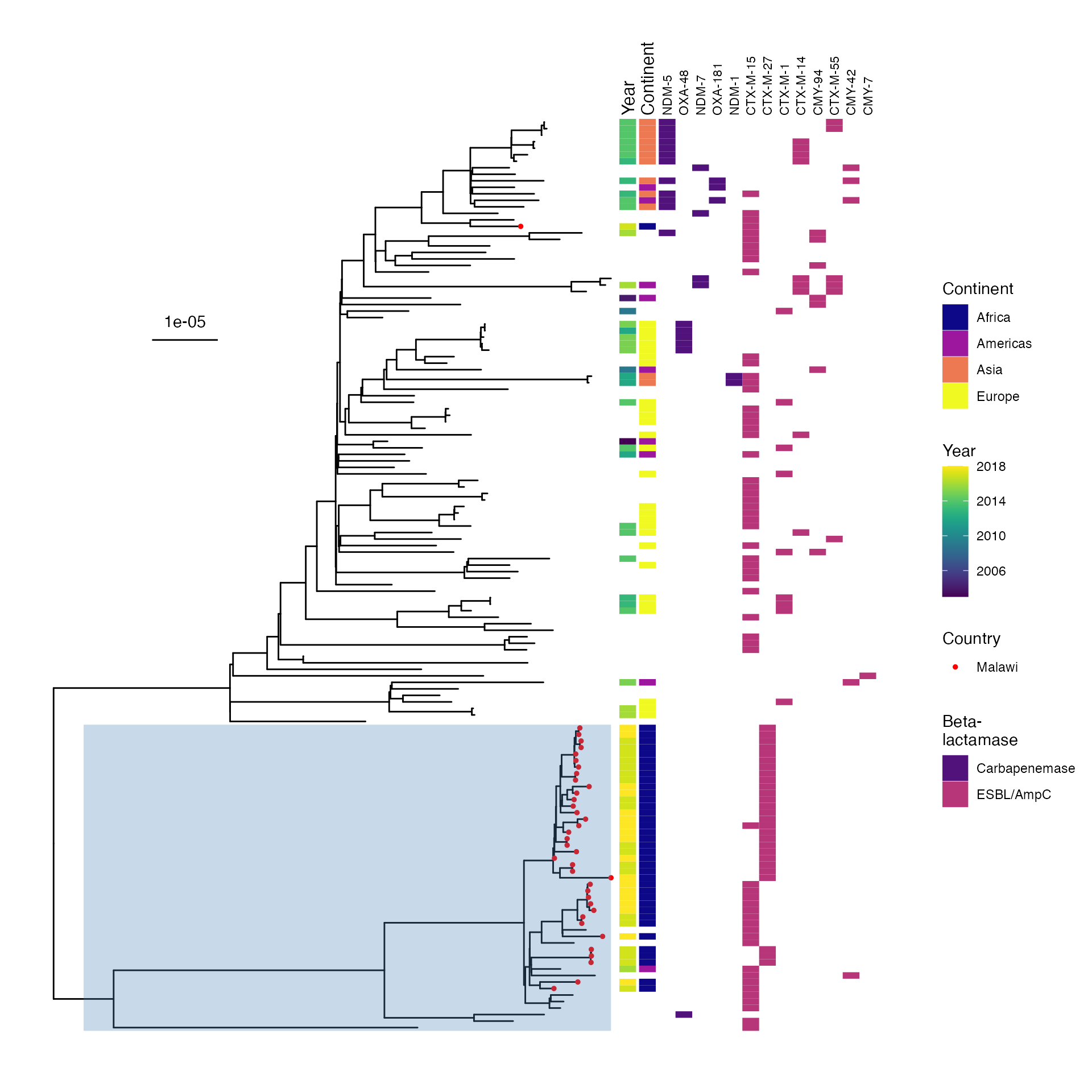
ST167 map-to-reference global maximum likelihood, midpoint rooted tree
if (write_figs) {

ggsave(here("figures/ecoli-genomics/st167_globaltreeplot.svg"),
       st167_globaltree_plot, width = 8, height = 10)

ggsave(here("figures/ecoli-genomics/st167_globaltreeplot.pdf"),
       st167_globaltree_plot, width = 8, height = 10)
}
tree_subset(
  btESBL_ecoli_globalst167_tree, 142, levels_back = 0) -> st167_subtree

esbl_cpe.ariba %>%
  subset(sample %in% st167_subtree$tip.label) %>%
  as.data.frame() ->
esbl_cpe.ariba167_subset

esbl_cpe.ariba167_subset[
  c(TRUE, apply(esbl_cpe.ariba167_subset[-1], 2, function(x) !all(is.na(x))))
] ->
esbl_cpe.ariba167_subset


btESBL_ecoli_st167_plasmids %>%
  bind_rows(
    btESBL_plasmidreplicons %>%
      mutate(
        ref_seq = gsub("\\..*$", "", ref_seq),
        ref_seq = gsub("_.*$", "", ref_seq),
        ref_seq = gsub("^FIA", "IncFIA", ref_seq)
      ) %>%
      filter(species == "E. coli") %>%
      select(-species) %>%
      rename(name = lane)
  ) %>%
  filter(grepl("Inc", ref_seq)) %>%
  filter(name %in% st167_subtree$tip.label) %>%
  unique() %>%
  group_by(ref_seq) %>%
  mutate(n = n()) %>%
  filter(n > 2) %>%
  ungroup() %>%
  select(-n) %>%
  arrange(fct_infreq(ref_seq)) %>%
  pivot_wider(
    id_cols = name,
    names_from = ref_seq,
    values_from = ref_seq,
    values_fn = function(x) {
      return("Present")
    },
    values_fill = NA_character_
  ) %>%
  as.data.frame() -> st167_plasm_onehot_subset

rownames(st167_plasm_onehot_subset) <- st167_plasm_onehot_subset$name

cont_cols <- viridis_pal(option = "plasma")(4)
names(cont_cols) <- c("Africa","Americas", "Asia","Europe")

  (
  (
  (ggtree(st167_subtree, size = 0.3) %<+% (select(st167_metadata, accession, Country) %>% mutate(Country = if_else(Country == "Malawi", "Malawi",NA_character_)))  %>%
     gheatmap(
       select(st167_metadata, `Year`),
       font.size = 4,
       width = 0.06,
       colnames_position = "top",
       color = NA,
       colnames_offset_y = 0,
       colnames_angle = 90,
       hjust = 0
     )  +
     scale_fill_viridis(name = "Year", limits = c(1978,2020),
                        na.value = "white") +
     new_scale_fill()) %>%
    gheatmap(
      select(st167_metadata, Continent),
      font.size = 4,
      width = 0.06,
      colnames_position = "top",
      color = NA,
      colnames_offset_y = 0,
      colnames_angle = 90,
      offset = 0.000005,
      hjust = 0
    ) +
    scale_fill_manual(values = cont_cols,
                      name = "Continent",
                      na.translate =
                      FALSE) +
      geom_point2(aes(subset = as.numeric(label) < 95 & !isTip), size = 1) +
    geom_tippoint(aes(color = Country), na.rm = TRUE, size = 1) +
    scale_color_manual(values  = "red", na.translate = FALSE) +
    new_scale_fill()
) %>%
  gheatmap(
    select(esbl_cpe.ariba167_subset, -sample),
    font.size = 2.5,
    width = 0.06*(ncol(esbl_cpe.ariba167_subset) - 1),
    colnames_position = "top",
    color = NA,
    colnames_offset_y = 0,
    colnames_angle = 90,
    offset = 0.00001,
    hjust = 0
  ) + scale_fill_manual(values = viridis_pal(option = "magma")(5)[c(2,3)],
                        na.translate = FALSE,
                        name = "Beta-\nlactamase") +
      new_scale_fill()
    ) %>%   gheatmap(
    select(st167_plasm_onehot_subset, -name),
    font.size = 2.5,
    width = 0.045*(ncol(st167_plasm_onehot_subset) - 1) + 0.1,
    colnames_position = "top",
    color = NA,
    colnames_offset_y = 0,
    colnames_angle = 90,
    offset = 0.000029,
    hjust = 0
  ) + scale_fill_manual(values = viridis_pal(option = "cividis")(7)[2],
                        na.translate = FALSE,
                        name = "Plasmid\nreplicon") +
  ylim(NA, 60) +
  geom_treescale(x = 0.00001, y = 60*0.666, offset = 1, width = 1e-5) ->
    st167_subtree_plot
#> Scale for fill is already present.
#> Adding another scale for fill, which will replace the existing scale.
#> Scale for fill is already present.
#> Adding another scale for fill, which will replace the existing scale.
#> Scale for fill is already present.
#> Adding another scale for fill, which will replace the existing scale.
#> Scale for fill is already present.
#> Adding another scale for fill, which will replace the existing scale.
#> Scale for y is already present.
#> Adding another scale for y, which will replace the existing scale.
if (write_figs) {
  btESBL_ecoli_st131_metadata %>%
    filter(Country != "Malawi") %>%
    write_csv(here("tables/ecoli-genomics/SUPP_T_st131_accession_numbers_and_metadata.csv"))
}
btESBL_ecoli_st131_metadata$malawi <- btESBL_ecoli_st131_metadata$Country == "Malawi"


btESBL_ecoli_st131_metadata$Continent <-
  countrycode(
    sourcevar = btESBL_ecoli_st131_metadata$Country,
    origin = "country.name",
    destination = "un.region.name"
  )
#> Warning: Some values were not matched unambiguously: Czech, Taiwan

btESBL_ecoli_st131_metadata$Continent[
  btESBL_ecoli_st131_metadata$Country == "Czech"
] <- "Europe"

btESBL_ecoli_st131_metadata$Continent[
  btESBL_ecoli_st131_metadata$Country == "Taiwan"
] <- "Asia"


rownames(btESBL_ecoli_st131_metadata) <- btESBL_ecoli_st131_metadata$Accession_number


btESBL_ecoli_st131_amr %>%
  pivot_wider(
    names_from = gene,
    values_from = gene,
    values_fn = length,
    values_fill = 0
  ) %>%
  mutate(across(everything(), as.character)) %>%
  as.data.frame() ->
amr.ariba131


rownames(amr.ariba131) <- amr.ariba131$name

btESBL_ecoli_st131_plasmids %>%
  filter(grepl("Inc", ref_seq)) %>%
  unique() %>%
  group_by(ref_seq) %>%
  mutate(n = n()) %>%
  filter(n >= 10) %>%
  ungroup() %>%
  select(-n) %>%
  arrange(fct_infreq(ref_seq)) %>%
  pivot_wider(
    id_cols = name,
    names_from = ref_seq,
    values_from = ref_seq,
    values_fn = function(x) {
      return("Present")
    },
    values_fill = NA_character_
  ) %>%
  as.data.frame() -> st131_plasm_onehot

rownames(st131_plasm_onehot) <- st131_plasm_onehot$name

esbl_cols <- viridis_pal(option = "magma")(5)[c(2, 3)]

names(esbl_cols) <- c("Carbapenemase", "ESBL/AmpC")

btESBL_ecoli_st131_amr %>%
  left_join(
    select(btESBL_NCBI_phenotypic_bl, allele_name, class),
    by = c("gene" = "allele_name")
  ) %>%
  mutate(class = case_when(
    grepl("CMY", name) ~ "ESBL/AmpC",
    class == "ESBL" ~ "ESBL/AmpC",
    TRUE ~ class
  )) %>%
  filter(class %in% c("ESBL/AmpC", "Carbapenemase")) %>%
  mutate(gene = gsub("_", "-", gene)) %>%
  arrange(class, fct_infreq(gene)) %>%
  pivot_wider(
    id_cols = "name",
    names_from = gene,
    values_from = class
  ) %>%
  as.data.frame() ->
#  select(-`TEM-15`) ->    # not in df?
esbl_cpe.ariba131
rownames(esbl_cpe.ariba131) <- esbl_cpe.ariba131$name

(
(
(ggtree(btESBL_ecoli_globalst131_tree, size = 0.2) %<+%
   (select(btESBL_ecoli_st131_metadata, Accession_number, Country) %>%
      mutate(Country = if_else(Country == "Malawi", "Malawi",NA_character_)))  %>%
    gheatmap(
      select(btESBL_ecoli_st131_metadata, `Year`),
      font.size = 4,
      width = 0.035,
      colnames_position = "top",
      color = NA,
      colnames_offset_y = 5,
      colnames_angle = 90,
      hjust = 0
    )  +
     scale_fill_viridis_c(name = "Year", limits = c(1965,2020),
                          na.value = "white") +
    new_scale_fill()) %>%
  gheatmap(
    select(btESBL_ecoli_st131_metadata, Continent),
    font.size = 4,
    width = 0.035,
    colnames_position = "top",
    color = NA,
    colnames_offset_y = 5,
    colnames_angle = 90,
    offset = 0.000005,
    hjust = 0
  ) +
  scale_fill_viridis_d(option = "plasma", name = "Continent",
                       na.translate = FALSE) +
  geom_tippoint(aes(color = Country), na.rm = TRUE, size = 1) +
  scale_color_manual(values  = "red", na.translate = FALSE) +
    new_scale_fill()
) %>%
  gheatmap(
  select(esbl_cpe.ariba131, -name),
  font.size = 2.5,
  width = (ncol(esbl_cpe.ariba131) -1)*0.03,
  colnames_position = "top",
  color = NA,
  colnames_offset_y = 5,
  colnames_angle = 90,
  offset = 0.0000103,
  hjust = 0
) + scale_fill_manual(values = esbl_cols,
                      na.translate = FALSE,
                      name = "Beta-\nlactamase") +
  new_scale_fill()
)   %>%   gheatmap(
    select(st131_plasm_onehot, -name),
    font.size = 2.5,
    width = 0.026*(ncol(st131_plasm_onehot) - 1) + 0.1,
    colnames_position = "top",
    color = NA,
    colnames_offset_y = 5,
    colnames_angle = 90,
    offset = 0.000059,
    hjust = 0
  ) + scale_fill_manual(values = viridis_pal(option = "cividis")(7)[2],
                        na.translate = FALSE,
                        name = "Plasmid\nreplicon") +
  ylim(NA, 1000) +
  geom_treescale(x = 0.00002, y = 1000*0.666, offset = 5, width = 0.00001)   +
  theme(legend.position = "none") +
      geom_point2(aes(subset = as.numeric(label) < 95 & !isTip), size = 0.5)  ->
  st131_globaltree_plot
#> Scale for fill is already present.
#> Adding another scale for fill, which will replace the existing scale.
#> Scale for fill is already present.
#> Adding another scale for fill, which will replace the existing scale.
#> Scale for fill is already present.
#> Adding another scale for fill, which will replace the existing scale.
#> Scale for fill is already present.
#> Adding another scale for fill, which will replace the existing scale.
#> Scale for y is already present.
#> Adding another scale for y, which will replace the existing scale.

st131_globaltree_plot
#> Warning in FUN(X[[i]], ...): NAs introduced by coercion
#> Warning in FUN(X[[i]], ...): NAs introduced by coercion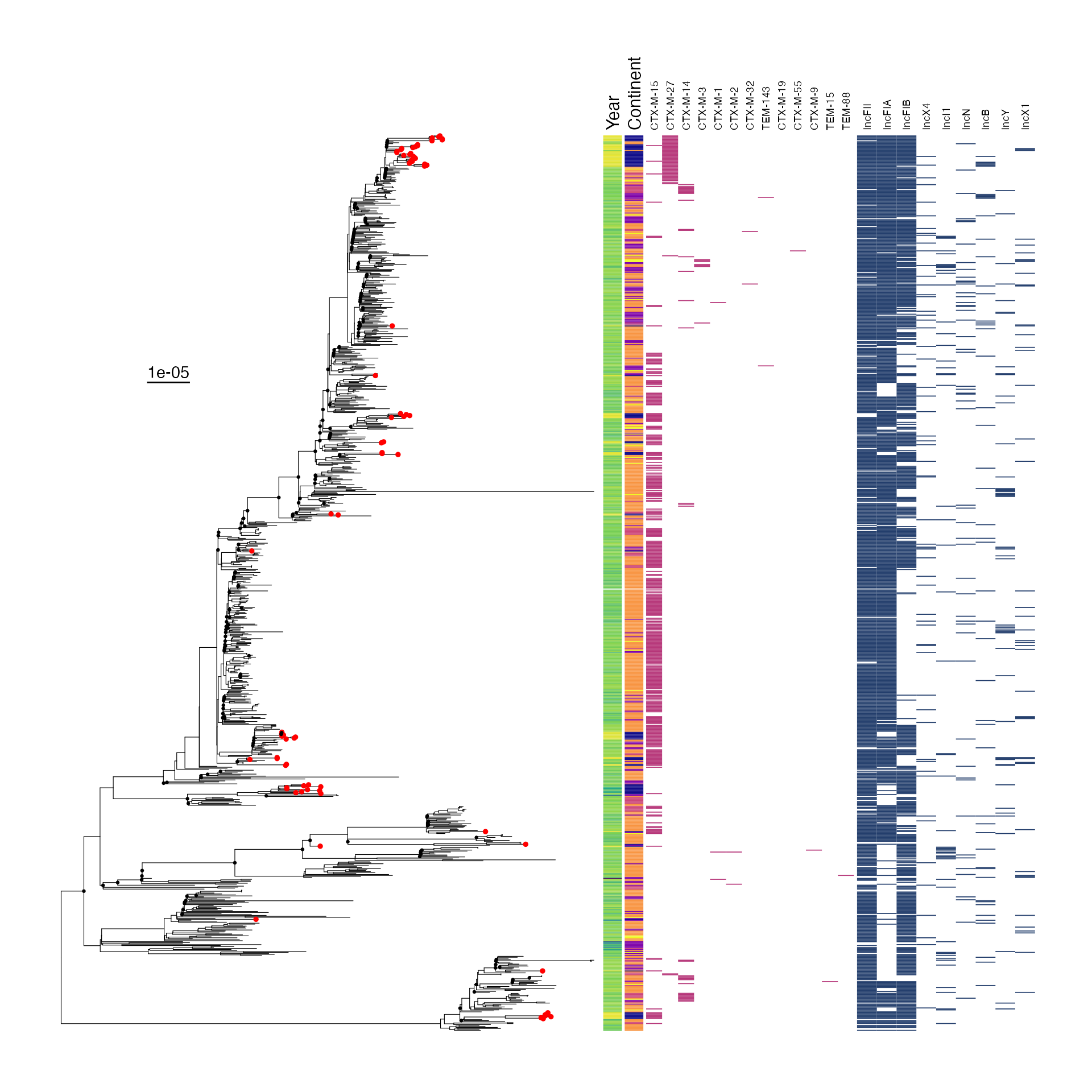
ST131 map-to-reference global maximum likelihood, midpoint rooted tree
st410_subtree_plot + st167_subtree_plot  + st131_globaltree_plot +
  plot_layout(widths = c(1,1.5),
              design = "AAAAACCCCCCCC
                        BBBBBCCCCCCCC") +
plot_annotation(tag_levels = "A") +
plot_layout(guides = "collect") -> st410_167_131_subtree_plot

st410_167_131_subtree_plot
#> Warning in FUN(X[[i]], ...): NAs introduced by coercion

#> Warning in FUN(X[[i]], ...): NAs introduced by coercion

#> Warning in FUN(X[[i]], ...): NAs introduced by coercion

#> Warning in FUN(X[[i]], ...): NAs introduced by coercion

#> Warning in FUN(X[[i]], ...): NAs introduced by coercion

#> Warning in FUN(X[[i]], ...): NAs introduced by coercion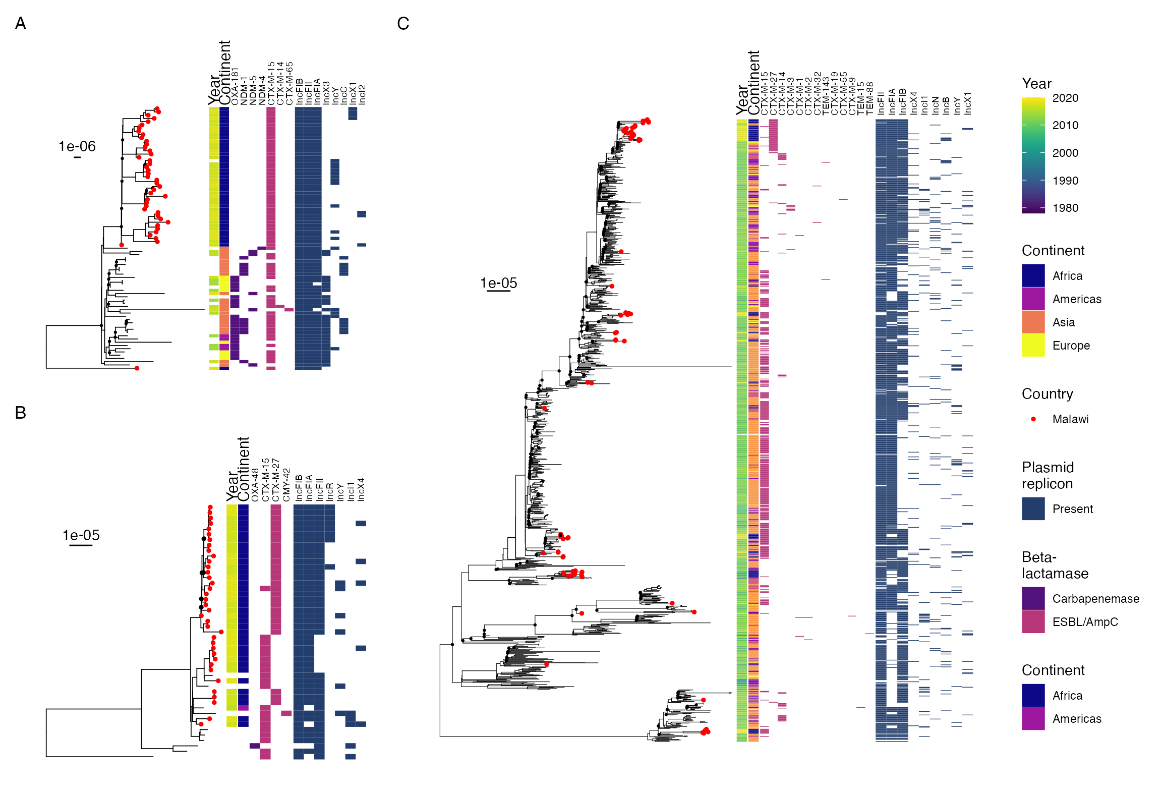
E. coli ST140 (A) and ST167 (B) subtrees and (C) ST131 tree showing ESBL/CPE genes and plasmid replicons
if (write_figs) {

ggsave(here("figures/ecoli-genomics/st410_167_131_subtreeplot.svg"),
       st410_167_131_subtree_plot, width = 12, height = 8.2)

ggsave(here("figures/ecoli-genomics/st410_167_131_subtreeplot.pdf"),
       st410_167_131_subtree_plot, width = 12, height = 8.2)
}
# ----------------------------------------------------------------------
# plot subtree of ST131

tree_subset(btESBL_ecoli_globalst131_tree, 1090) -> st131_subtree


esbl_cpe.ariba131 %>%
  subset(name %in% st131_subtree$tip.label) %>%
  as.data.frame() ->
esbl_cpe.ariba131_subset

esbl_cpe.ariba131_subset[
  c(TRUE, apply(esbl_cpe.ariba131_subset[-1], 2, function(x) !all(is.na(x))))
] ->
esbl_cpe.ariba131_subset


st131_plasm_onehot %>%
  subset(name %in% st131_subtree$tip.label) %>%
  as.data.frame() -> st131_plasm_onehot_subset


st131_plasm_onehot_subset[
  c(TRUE, apply(st131_plasm_onehot_subset[-1], 2, function(x) !all(is.na(x))))
] ->

st131_plasm_onehot_subset

(
  (
    (ggtree(tree_subset(btESBL_ecoli_globalst131_tree, 1090)) %<+%
      (select(btESBL_ecoli_st131_metadata, Accession_number, Country) %>%
        mutate(Country = if_else(Country == "Malawi",
          "Malawi", NA_character_
        ))) %>%
      gheatmap(
        select(btESBL_ecoli_st131_metadata, `Year`),
        font.size = 4,
        width = 0.035,
        colnames_position = "top",
        color = NA,
        colnames_offset_y = 0,
        colnames_angle = 90,
        hjust = 0
      ) +
      scale_fill_viridis_c(
        name = "Year", limits = c(1965, 2020),
        na.value = "white"
      ) +
      new_scale_fill()) %>%
      gheatmap(
        select(btESBL_ecoli_st131_metadata, Continent),
        font.size = 4,
        width = 0.03,
        colnames_position = "top",
        color = NA,
        colnames_offset_y = 0,
        colnames_angle = 90,
        offset = 0.0000008,
        hjust = 0
      ) +
      scale_fill_viridis_d(
        option = "plasma", name = "Continent",
        na.translate = FALSE
      ) +
      geom_tippoint(aes(color = Country), na.rm = TRUE, size = 1) +
      scale_color_manual(values = "red", na.translate = FALSE) +
      new_scale_fill()
  ) %>%
    gheatmap(
      select(esbl_cpe.ariba131_subset, -name),
      font.size = 2.5,
      width = (ncol(esbl_cpe.ariba131_subset) - 1) * 0.03,
      colnames_position = "top",
      color = NA,
      colnames_offset_y = 0,
      colnames_angle = 90,
      offset = 0.0000015,
      hjust = 0
    ) + scale_fill_manual(
      values = esbl_cols,
      na.translate = FALSE,
      name = "Beta-\nlactamase"
    ) +
    new_scale_fill()
) %>% gheatmap(
  select(st131_plasm_onehot_subset, -name),
  font.size = 2.5,
  width = 0.026 * (ncol(st131_plasm_onehot_subset) - 1) + 0.1,
  colnames_position = "top",
  color = NA,
  colnames_offset_y = 0,
  colnames_angle = 90,
  offset = 0.0000032,
  hjust = 0
) + scale_fill_manual(
  values = viridis_pal(option = "cividis")(7)[2],
  na.translate = FALSE,
  name = "Plasmid\nreplicon"
) +
  ylim(NA, 80) +
  geom_treescale(x = 0.000001, y = 55, offset = 1, width = 0.000001) +
  geom_point2(aes(subset = as.numeric(label) < 95 & !isTip), size = 0.5) ->
st131_subtree_plot
#> Scale for fill is already present.
#> Adding another scale for fill, which will replace the existing scale.
#> Scale for fill is already present.
#> Adding another scale for fill, which will replace the existing scale.
#> Scale for fill is already present.
#> Adding another scale for fill, which will replace the existing scale.
#> Scale for fill is already present.
#> Adding another scale for fill, which will replace the existing scale.
#> Scale for y is already present.
#> Adding another scale for y, which will replace the existing scale.

st131_subtree_plot
#> Warning in FUN(X[[i]], ...): NAs introduced by coercion

#> Warning in FUN(X[[i]], ...): NAs introduced by coercion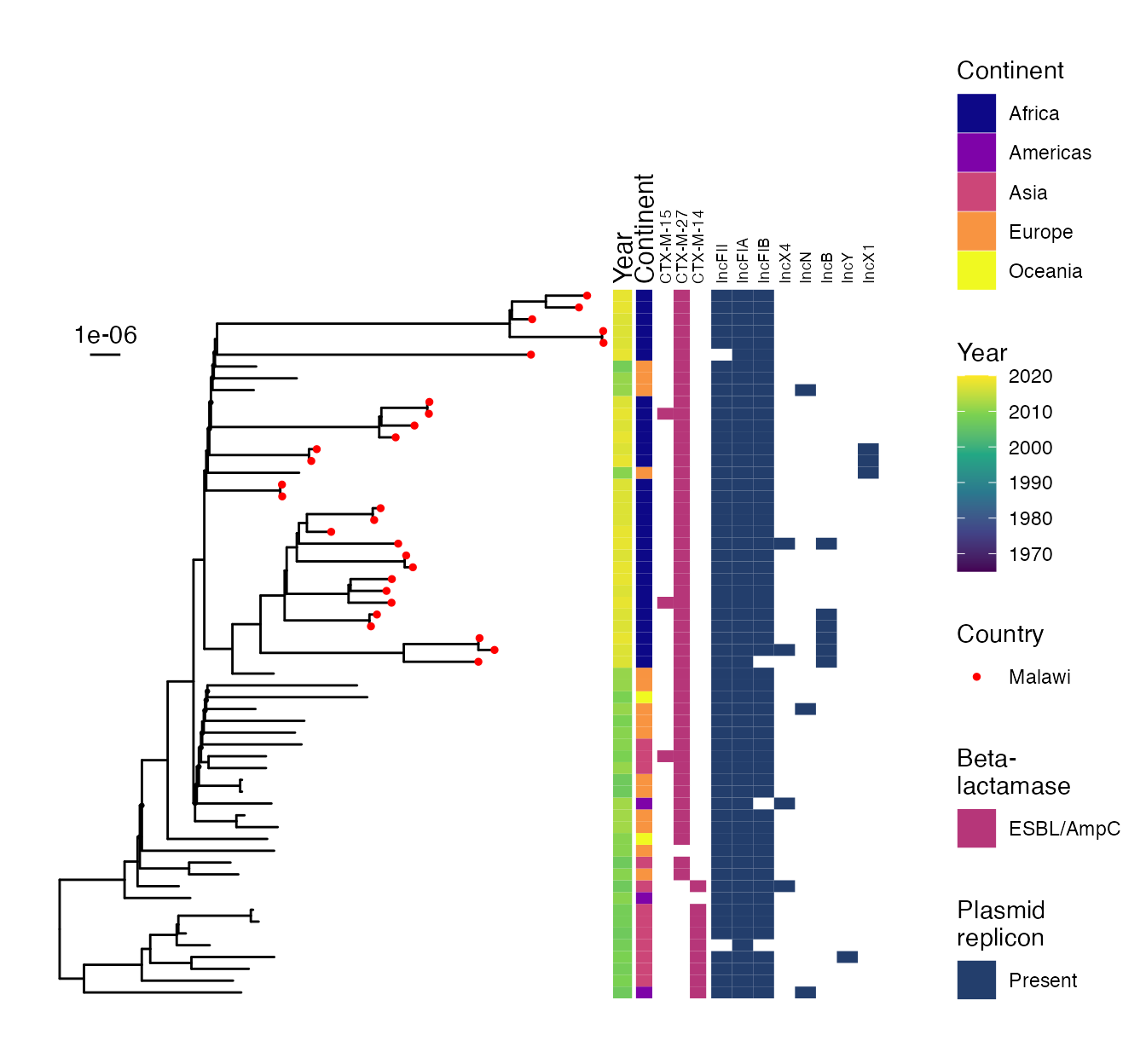
E. coli ST131 subtree showing detail of CTX-M-27 isolates and one area in which Malawian isolates are monophyletic
Reproducibility - packages, R version and OS used
sessionInfo()
#> R version 4.3.1 (2023-06-16)
#> Platform: aarch64-apple-darwin20 (64-bit)
#> Running under: macOS Sonoma 14.0
#>
#> Matrix products: default
#> BLAS:   /Library/Frameworks/R.framework/Versions/4.3-arm64/Resources/lib/libRblas.0.dylib
#> LAPACK: /Library/Frameworks/R.framework/Versions/4.3-arm64/Resources/lib/libRlapack.dylib;  LAPACK version 3.11.0
#>
#> locale:
#> [1] en_GB.UTF-8/en_GB.UTF-8/en_GB.UTF-8/C/en_GB.UTF-8/en_GB.UTF-8
#>
#> time zone: Europe/London
#> tzcode source: internal
#>
#> attached base packages:
#> [1] stats     graphics  grDevices utils     datasets  methods   base
#>
#> other attached packages:
#>  [1] viridis_0.6.4      viridisLite_0.4.2  countrycode_1.5.0  ggstance_0.3.6
#>  [5] scales_1.2.1       here_1.0.1         patchwork_1.1.3    kableExtra_1.3.4
#>  [9] ggnewscale_0.4.9   lubridate_1.9.3    blantyreESBL_1.4.1 stringr_1.5.0
#> [13] forcats_1.0.0      ggplot2_3.4.3      readr_2.1.4        tidyr_1.3.0
#> [17] dplyr_1.1.3        phytools_1.9-16    maps_3.4.1         ape_5.7-1
#> [21] ggtree_3.9.1       tidytree_0.4.5
#>
#> loaded via a namespace (and not attached):
#>  [1] mnormt_2.1.1            gridExtra_2.3           phangorn_2.11.1
#>  [4] rlang_1.1.1             magrittr_2.0.3          compiler_4.3.1
#>  [7] systemfonts_1.0.4       vctrs_0.6.3             combinat_0.0-8
#> [10] quadprog_1.5-8          rvest_1.0.3             crayon_1.5.2
#> [13] pkgconfig_2.0.3         fastmap_1.1.1           labeling_0.4.3
#> [16] utf8_1.2.3              rmarkdown_2.25          tzdb_0.4.0
#> [19] ragg_1.2.5              bit_4.0.5               purrr_1.0.2
#> [22] xfun_0.40               cachem_1.0.8            aplot_0.2.2
#> [25] clusterGeneration_1.3.8 jsonlite_1.8.7          highr_0.10
#> [28] parallel_4.3.1          R6_2.5.1                RColorBrewer_1.1-3
#> [31] bslib_0.5.1             stringi_1.7.12          jquerylib_0.1.4
#> [34] numDeriv_2016.8-1.1     Rcpp_1.0.11             iterators_1.0.14
#> [37] knitr_1.44              optimParallel_1.0-2     Matrix_1.6-1.1
#> [40] igraph_1.5.1            timechange_0.2.0        tidyselect_1.2.0
#> [43] rstudioapi_0.15.0       yaml_2.3.7              doParallel_1.0.17
#> [46] codetools_0.2-19        lattice_0.21-8          tibble_3.2.1
#> [49] treeio_1.26.0           withr_2.5.1             coda_0.19-4
#> [52] evaluate_0.22           gridGraphics_0.5-1      desc_1.4.2
#> [55] xml2_1.3.5              pillar_1.9.0            foreach_1.5.2
#> [58] ggfun_0.1.3             generics_0.1.3          vroom_1.6.4
#> [61] rprojroot_2.0.3         hms_1.1.3               munsell_0.5.0
#> [64] glue_1.6.2              scatterplot3d_0.3-44    lazyeval_0.2.2
#> [67] tools_4.3.1             webshot_0.5.5           fs_1.6.3
#> [70] fastmatch_1.1-4         grid_4.3.1              plotrix_3.8-2
#> [73] colorspace_2.1-0        nlme_3.1-162            cli_3.6.1
#> [76] textshaping_0.3.6       fansi_1.0.5             expm_0.999-7
#> [79] svglite_2.1.2           gtable_0.3.4            yulab.utils_0.1.0
#> [82] sass_0.4.7              digest_0.6.33           ggplotify_0.1.2
#> [85] farver_2.1.1            memoise_2.0.1           htmltools_0.5.6.1
#> [88] pkgdown_2.0.7           lifecycle_1.0.3         httr_1.4.7
#> [91] bit64_4.0.5             MASS_7.3-60